Using Tables in Excel

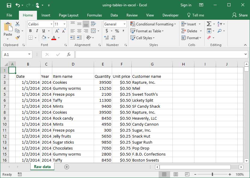
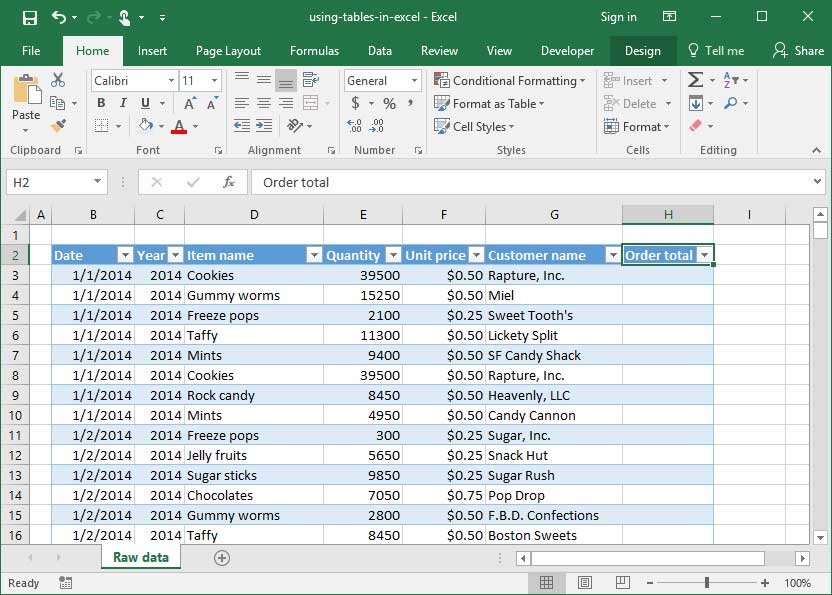
Just about all of the data we enter into Excel is structured in table format — meaning that it's organized in a grid of columns and rows. Some of the time, this data takes the form of a free-flowing analysis, where rows, columns, and cells are combined together to perform a calculation, estimation, or prediction. But sometimes, Excel is just used to organize large quantities of data. For example, the below spreadsheet tracks orders placed by SnackWorld's customers from 2014-2016. Every line of the spreadsheet contains directly comparable data: information on one order, like the order date, item name, quantity, and unit price.

In this latter case, Excel provides an incredibly handy feature that helps us organize and manipulate similar rows of data more effectively: Tables. Not to be confused with 'tables'-with-a-lower-case-T, our generic term for data sets organized into rows and columns, Tables-with-a-capital-T are a specific Excel feature. Let's dive in and take a look at what they can do!

Organizing the data

Before we can create a Table, we'll need to make sure that our source data set is formatted properly. Here are the main requirements we'll be looking at before we dive in:

Our source data must:

• Be structured in row-column format, with each row containing information on one line-item that is directly comparable to all other line-items;
• Have a unique, easily understood heading for each column of data;
• Avoid blank rows in between lines of data (e.g., be one cohesive table with no gaps or inconsistencies);
• Have columns that contain similar data types (e.g., each column should describe one property of data that is directly comparable across the entire column); and
• Not contain any subtotal or total rows. Each line should be a comparable piece of data, not a summary line or total.

Our source data set below fits all of the above criteria, so, once we've double-checked to ensure that everything is ready to go, we can get started creating our table.

Making the Table

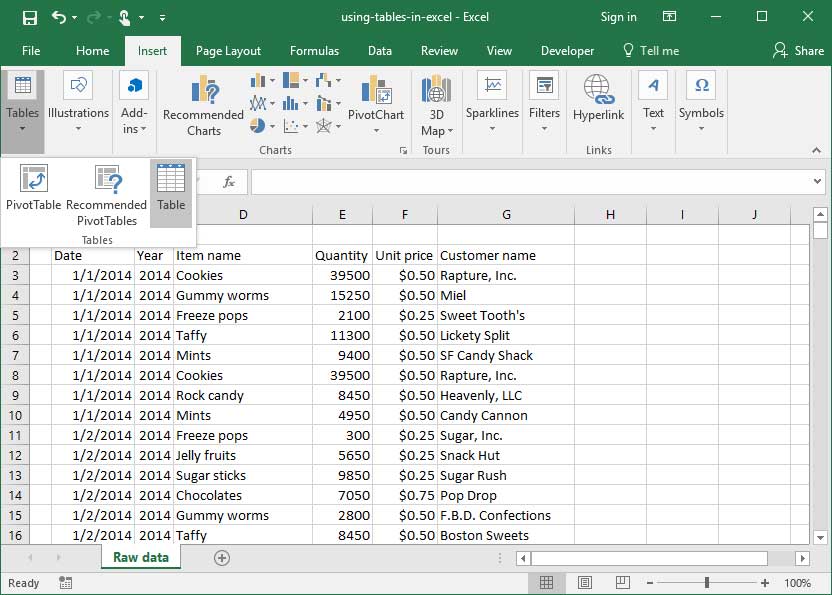
Once our data is well-structured, creating a table is easy! We'll simply select our entire source data set, head to the Insert tab on the ribbon, and hit the Table button:

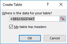
Since the source data we've selected includes the headers of our table, we'll make sure the "My table has headers" box is checked in the dialogue that appears, then press OK:

The first benefit of structuring data as a Table immediately becomes apparent: Excel has automatically added beautiful headers and row striping to our data so that it's easy to read and looks fantastic:

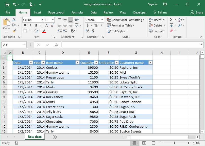
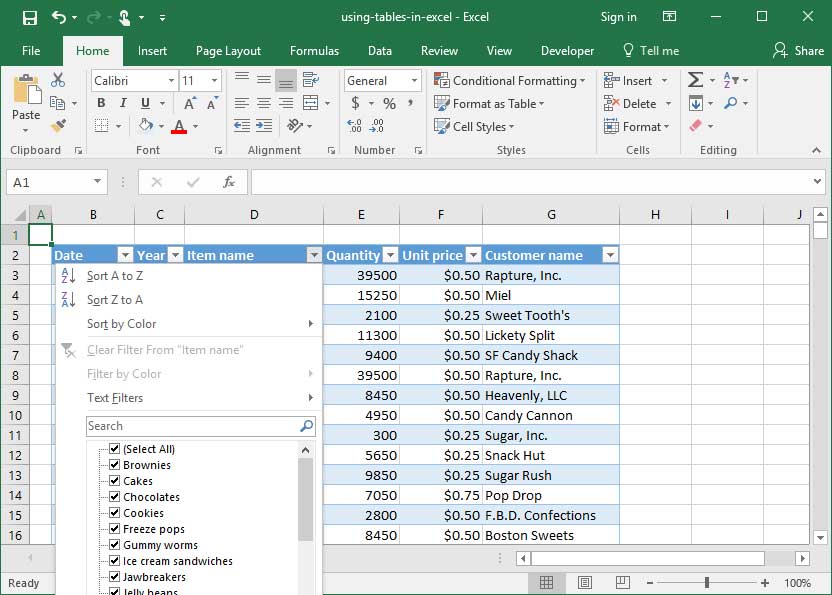
Additionally, notice that Excel has added drop-down arrows below each header of our Table. Click one of those arrows to bring up a sorting and filtering menu that provides a bevy of built-in functionality for alphabetizing, data filtering, and more — no additional Sort or Filter commands required!

Those are the basics of Table creation, but there are a few other important advantages to structuring our data as a Table that make this feature even more useful. Let's take a look!

Easy totaling

First of all, structuring our data as a Table allows us to total it quickly and easily. Simply head to the Design tab on the Ribbon, and check the box that says "Total Row" in the Table Style Options section:

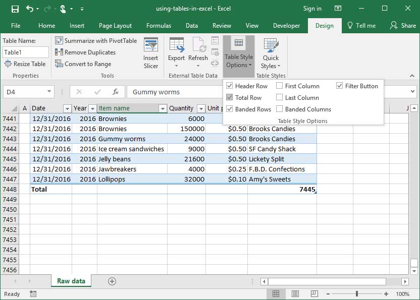
A grand total row is automatically added to the bottom of our table. Note that there's a dropdown next to each cell on this total row, which can be switched to use various functions including SUM, COUNT, and AVERAGE:

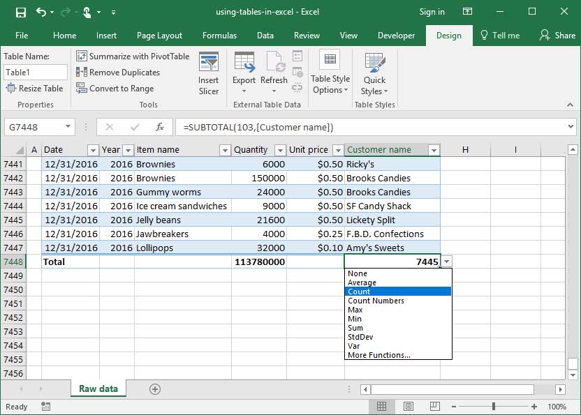
This makes it very easy to perform SUMs, COUNTs, and more of the full data table range!

Adding rows

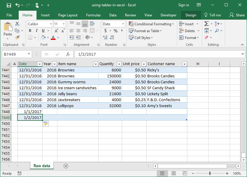
Note that if we scroll to the bottom of our Table and begin typing an additional row of data, Excel automatically formats our input as a new row of the Table in question:

Additionally, if we copy and paste data into a Table, it will automatically be expanded to fit the data that is pasted in.

Same-row references and auto-fills

Our data set currently contains a Quantity column and a Unit price column, but doesn't have an Order total column. We could pretty easily create one by multiplying Quantity by Unit price.

Let's start by creating a new column. To do so, we'll position our cursor in Cell H2 and typing a new column name: Order total. When we press Return, notice that Excel automatically adds a new column to our Table and formats it nicely — just like the rest of the data:

Now, with our cursor in Cell H3, let's start writing a formula to multiply Quantity by Unit price. We'll start with the = sign, then use the arrow keys on our keyboard to navigate to the cells we want to reference.

Notice that something unusual happens here: when we navigate our reference to the Quantity column, our formula bar doesn't reference Cell E3; rather, it reads:

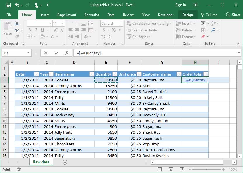
=[@Quantity]

This is a type of cell reference that we've never seen before. What's going on here?

It turns out that Tables allow us to make references to column names rather than just cell addresses. These two types of references are functionally equivalent, but referencing column names allows us to write easier-to-read formulas quickly and easily.

These column name references can only be used when referencing a Table cell on the same row as the source cell, and they're completed by preceding a column name with the @ symbol and enclosing it in brackets ([ and ]) like so:

=[@Quantity]

The above formula will pull whatever value sits in the Quantity column of the table in which the formula is being written on the same row as the source formula.

When the column name contains spaces, it must be enclosed within an additional set of brackets:

=[@[Unit price]]

Column references can also be used when constructing a formula outside of the referenced table like so:

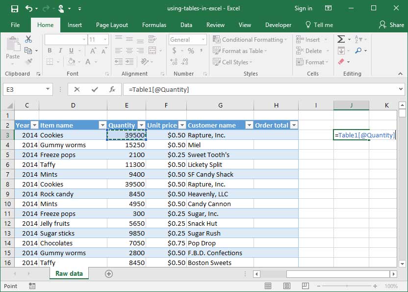
=Table1[@[Unit price]]

Note that this formula outputs the value in the referenced Table's Unit price column that appears on the same row as the referencing formula.

With this all in mind, let's complete our formula in the Order total column, which will reference both the Quantity and Unit price columns:

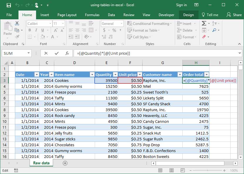
=[@Quantity]*[@[Unit price]]

When we press Return notice that Excel automatically copies our formula down to every cell in the Table. This is another important table feature: Autofill. Excel automatically fills in formulas for every Table row, when added or updated. No manual copy-and-paste work necessary!

Whole-column references

Tables also make referencing entire columns from outside the Table quick and easy. We can do so with the following syntax:

=TableName[Column Name])

For example, if we wanted to find the SUM of all values in our new Order total column, we could do so with the following formula:

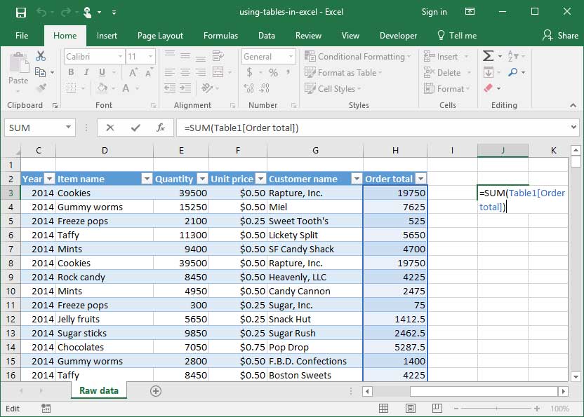
=SUM(Table1[Order total])
Output: $52,299,353

This approach has a number of advantages:

• First, writing the formula is easy. There are no cell references to deal with, so formulas summing up an entire column of data become extremely quick to construct.
• Second, the formula will automatically update when new rows are added to the Table. If new data is copied and pasted into the Table, or if new rows are added at the bottom, a whole-column referencing formula will automatically update to include the additions. This makes Tables a go-to data input choice when constructing dashboards in Excel. As the dashboards are updated with new data (which is either entered into a new line on the table in question; or copy-and-pasted in from an external source), all formulas will automatically update to include the entire Table — with any new information. Without Tables, dashboard formulas need to reference entire columns of data in Excel (e.g., E:E or E1:E99999), which can lead to massive computation times.

Use whole-column references on Tables whenever you're constructing a tool that needs to be updated frequently with new data.

Referencing headers

Finally, headers of a table can be referenced using the #Headers modifier like so:

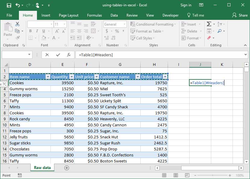
=Table1[#Headers]

This can be useful for simplifying formulas that reference the header row of a table, like VLOOKUP or INDEX MATCH.

Comments