How to filter data with autofilters in Excel

If you're working with a small table of data, oftentimes it just takes a couple of quick sorts to clean it up and make it readable for your users. But for larger spreadsheets — those with tens, hundreds, or thousands of rows — a little more firepower is often necessary when you're looking for specific data points.

For this, we use an Excel feature called filters. Filters are automated features built into Excel that will allow us to view a subset of our data based on criteria that we specify. This will make it much easier to isolate rows in a table without scrolling through huge amounts of data.

Defining the problem

Take a look at the spreadsheet below, which shows SnackWorld's sales numbers by customer and month.

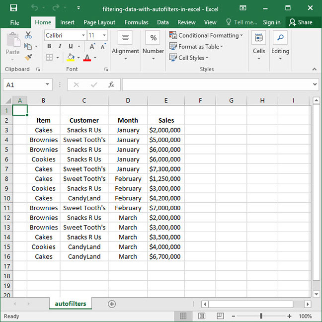
What would we do if we wanted to isolate a particular portion of this spreadsheet — for example, only show rows for which the Month is equal to February? One solution would be to sort our data using Excel's automated sorting features (for more information, check out our guide to sorting and alphabetization). But larger data sets will be difficult to comb through even after sorting.

Using basic autofilters

Enter autofilters. This Excel feature will allow us to narrow our data range based to a smaller set of rows based on criteria we select. To get started, place your cursor anywhere within the data table you're working with, and press the Filter button located on the Data ribbon. You'll see small arrows appear next to your column headers, like so:

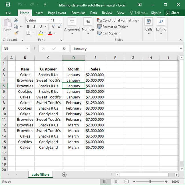
When you see these arrows, you'll know that you're now able to play around with filtering.

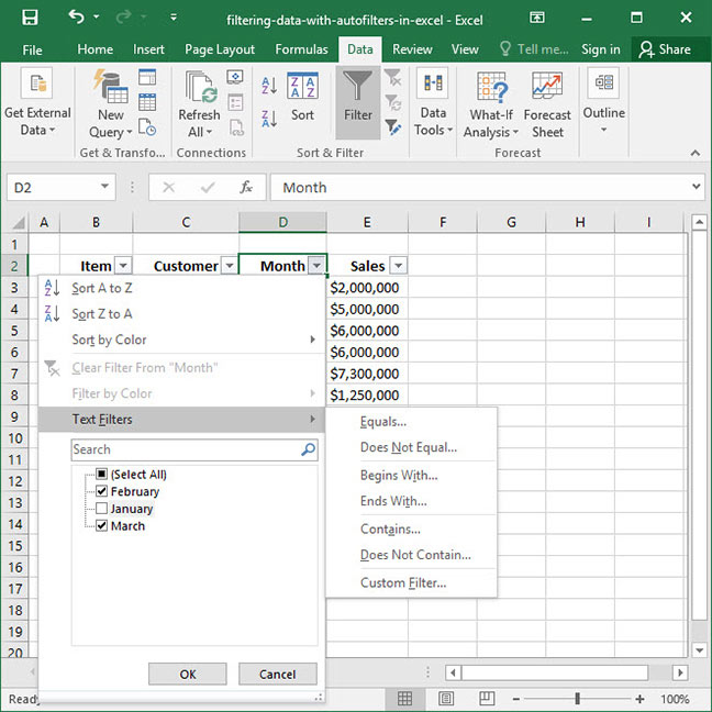
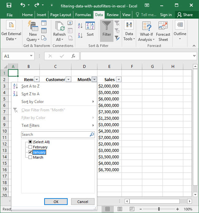
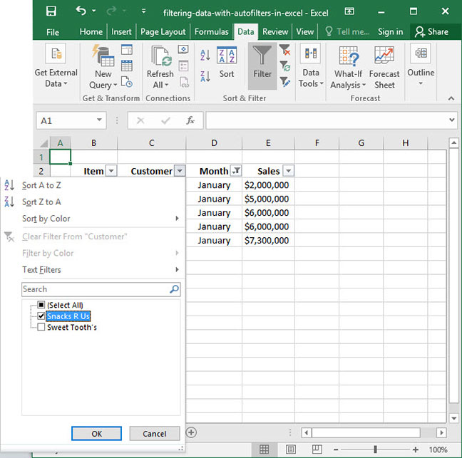
Let's go ahead and press the arrow button next to the Month column header. A filtering menu will appear that allows us to filter our data based on any number of criteria we select.

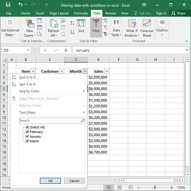
Let's review the key features of the filtering menu. First, you'll notice that there are Sort A to Z and Sort Z to A shortcuts at the top of the menu. These allow us a quick and easy way to sort our data without accessing the Data section of the ribbon.

Next, notice that all the values that appear within the Month column of our table appear in the bottom dialogue with check marks next to them. Let's try unchecking January and March (leaving only February remaining), like so:

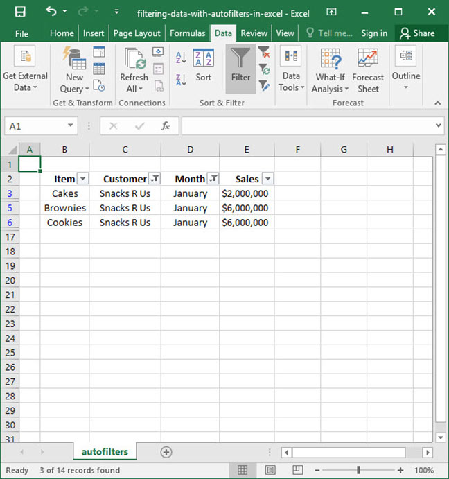
Finally, we'll press the OK button to commit our changes. Notice that our table has changed: only rows for which the month is equal to February are now showing!

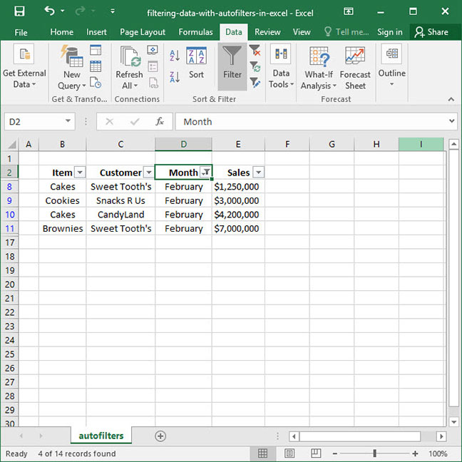
The beauty of this tool is that our actual table has not changed at all. All of the data for January and March is preserved; it's just been hidden by Excel so that we can read our data set more easily.

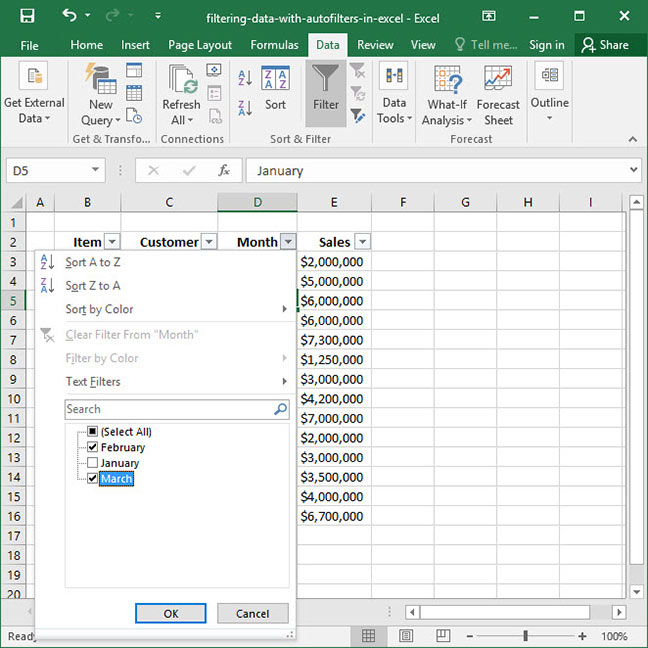
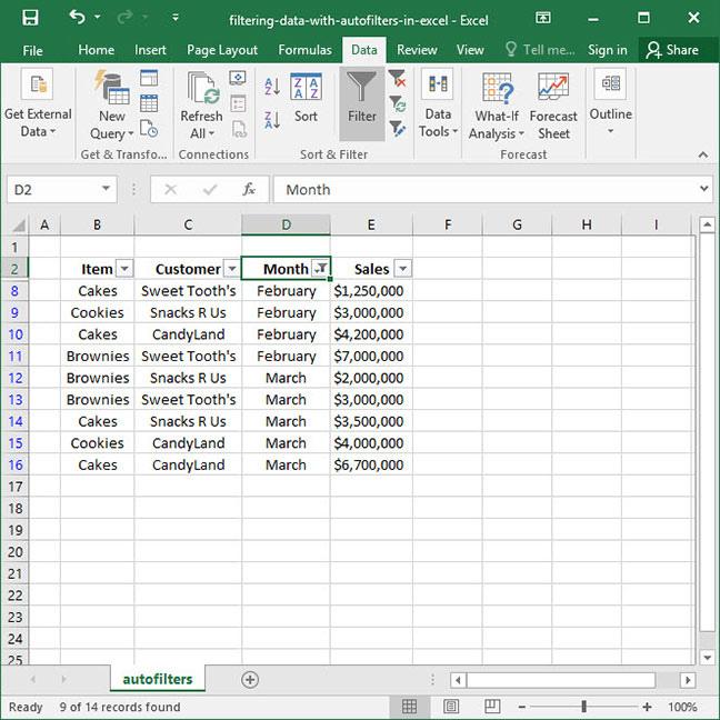
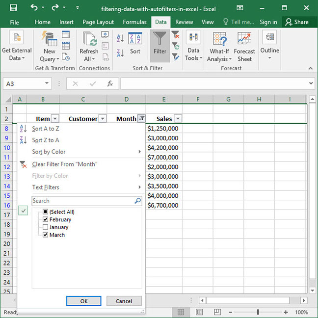
The other great feature of filters is that we can select as many or as few data points as we want. Open the filtering menu back up on the Month column, and check the box next to March, like so:

Finally, press OK. You'll see that since both February and March are checked, our table now shows data for both of those months:

Modifying filtered data

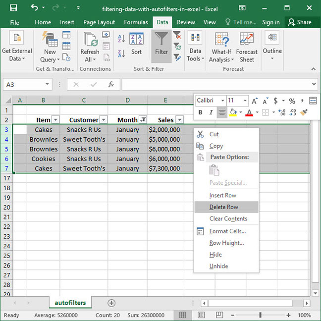
One of Excel's most convenient features is that it only modifies data that has been filtered, and excludes everything else. So if we wanted to delete all the rows in which Month equals January, we could just filter for January-only rows, select them all, and delete them from our sheet, like so:

Clearing filters

So we've filtered our data and done what we need with it; but afterwards, how do we get our full dataset back? The answer is simple: Excel's Clear filter option.

When working with a data set in Excel, a small "filter" icon next to the column header () will indicate that a column has been filtered. In the example below, this symbol appears next to the Month column. To clear the filter on this column, click the icon, then use the Clear filter option:

After clicking this button, the filter will clear and our dataset will be back to normal:

The Search feature

Our filters are working great when we only have three months to select between. But what if our table were so big that it was difficult to find values to select?

Fortunately, Excel has a handy Search feature to deal with this problem. Let's open our Month filtering menu back up, and test out the search box provided above the list of months. Enter the characters Jan into the box, and you'll see that Excel automatically filters the list of months down to those that contain the string of text we entered:

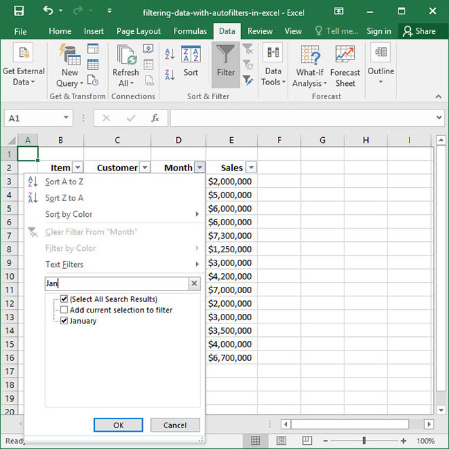
At this point, checking the box next to January and pressing OK will clear all other filters, so that just January values show in our table. Or, check the box next to the Add current selection to filter option, and January will be added to the list of boxes that are already checked.

Multiple filters in Excel

Above, we looked at how to apply a basic filter to one column. But it's also possible to apply multiple filters — to multiple columns — at once in Excel. Find out how below.

First, let's apply a Month filter to show only rows in January, like so:

Now, let's say we wanted to only show orders from the customer called Snacks R Us. We can narrow down our data set even further by applying another filter, this time to the Customer column. Click the arrow icon next to the Customer column header to open up the Customer filtering screen:

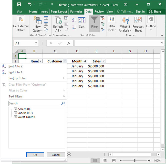
Click the checkbox next to (Select all) to deselect everything, then click the checkbox next to Snacks R Us to ensure that they are the only customer selected:

Finally, press OK. Like magic, our list is filtered even more — we now see only January sales to Snacks R Us!

We can apply as many filters as needed onto our data set, filtering across multiple columns with multiple criteria. Just remember: whenever you're done, be sure to Clear filters on every column you've modified. Look out for those filter icons () to give you a heads-up for when you accidentally miss one. You can also use the Clear all filters command in the Ribbon to clear everything at once:

Advanced filters

Let's open up our Sales filtering menu, which filters based on the dollar sales amount specified in our table. Once the menu is open, hover over the Number filters option to show some more advanced filtering options:

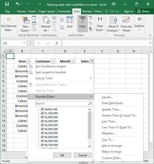
Excel automatically tailors these advanced filtering options to the type of column that we're filtering on — in this case, a Numerical column. This menu will change automatically depending on the type of column with which we're working. Try opening up the advanced filtering menu on columns of these types to see what Excel will allow you to do with them:

• Numerical columns use advanced number filters, which allow you to filter based on 'equal' and 'does not equal' criteria; 'greater than', 'less than', and 'between' criteria; 'above average' and 'below average' criteria, and 'Top 10' value lists.
• Text columns use advanced text filters, which allow you to filter based on 'equal' and 'does not equal' criteria; 'begins with' and 'ends with' criteria; and 'contains' and 'does not contain' criteria.
• Date columns use advanced date filters, which allow you to filter based on 'before', 'after', and 'between' criteria; daily, weekly, monthly, quarterly, and yearly comparisons; 'year to date' criteria; and other individual time periods.

Those are the basics of using autofilters — including filters on multiple columns — in Excel! Questions or comments on the process? Be sure to let us know in the Comments section below.

Comments