Excel's SUMIF function

Many Excel users think that the IF function is the program's most powerful conditional tool. But it turns out that there are a whole class of even more powerful functions that allow you to perform conditional calculations on large ranges of data. To begin, we'll start by learning about the most simple of these: the SUMIF function.

Excel's SUMIF allows you to perform a SUM of a particular range of data, but only include numbers for which certain conditions are met. For example, say we have a database of sales by product category. We can take the SUM of all products in the category Candy by using a SUMIF function. Let's take a look at how it looks.

Defining the problem

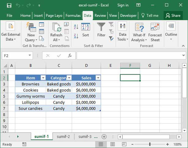
Take a look at the following table, which shows SnackWorld sales for various types of item, including Brownies, Cookies, and Gummy Worms:

Let's say we want to find out how much money SnackWorld made from selling all items in the Baked Goods category. With a large spreadsheet, it would be a pain to sum these all up manually. Fortunately, we have the SUMIF function to assist us.

Using SUMIF

The formula for the SUMIF function is as follows:

=SUMIF(range, criteria, sum_range (optional))

Notice that the sum_range argument at the end of the function is optional. We'll use that argument with most of our applications of SUMIF, but first, let's take a look at what happens when we leave it off.

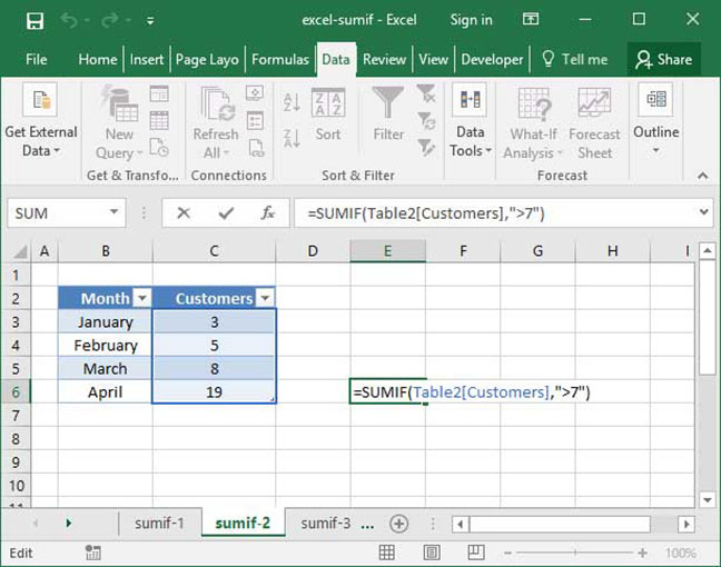
With just two arguments, the SUMIF argument is very simple. It takes the sum of every number in the given range, provided that the given criteria for that number is met. For example, consider the following formula, which sums up customer numbers by month:

=SUMIF(C3:C6, ">"&7)
Output: 27

What's going on here? First, Excel looks at the cells C3:C6, which it knows we want to take the SUM of. However, there's a condition: Excel looks at the criteria column to see whether there are any cells that we should exclude from the SUM. As it turns out, the criteria we've set here is ">"&7. This means that Excel should only include cells whose value is greater than or equal to 7 in our SUMIF. Therefore, the only cells it includes are C5 and C6 — which contain the values 8 and 19. The final output is 27.

What's with the quotes and ampersand around the ">"&7? It turns out that the condition argument takes a string, not a logical expression. It's a bit confusing for beginners, but that's just the way it's built! We enclose the > sign in quotes (" ") to turn it into a string that Excel recognizes. We then use the ampersand (&) sign to join this string to a regular number, 7, which we also want to include in our conditional statement.

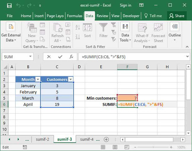
Instead of writing the condition as ">"&7, we could also write it as ">7", including the number 7 as a part of the string we provide to the function. However, we find that it's easier to always use the notation containing &, as it'll make things simpler when we include cell references in our conditionals. For example, take a look at the following formula, where we've included a cell reference rather than a hard-coded number in the condition:

=SUMIF(C3:C6, ">"&F5)
Output: 27

See how we use the & sign to join the ">" string with a cell reference to F5? If we included the argument F5 within the quotes, the formula wouldn't work, because Excel would treat it as a string rather than a cell reference.

SUMIF with three arguments

What we've done so far is nice, but not particularly useful. Why would we only want to take the sum of Customers if the number of customers in any given month is greater than seven?

That's when the third argument of SUMIF comes in: sum_range. This argument will allow us to take the sum of a range that's different from our condition. In other words, SUMIF will take the SUM of everything in sum_range, but only if the given condition is met for everything within the range provided.

To see how this works, let's take a look at the spreadsheet from the beginning of this tutorial, which lists product sales by item and category:

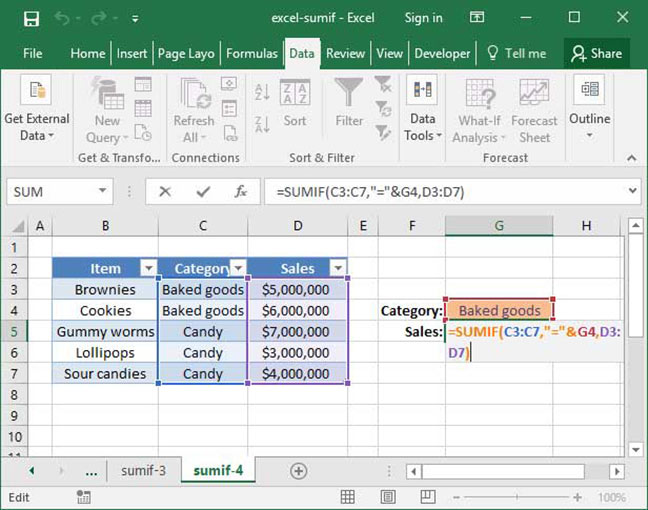
Let's construct a SUMIF formula with three arguments to take the SUM of everything in the Baked Goods category:

=SUMIF(C3:C7,"="&G4,D3:D7)
Output: $11,000,000

As you can see, the SUMIF function takes the sum of everything our our sum_range (D3:D7), but only if the corresponding cells in our range (C3:C7) meet our stated condition ("="&G4). Since cell G4 contains the phrase "Baked goods", only cells D3 and D4 are included in the sum, for a total of $11,000,000.

There's another shortcut we can use here: when using the = sign, we don't need to include the "="& part of our condition. If Excel doesn't see any logical operators, it will assume that we are trying to ensure that the value in a particular cell is equal to what we have in our range. So, the above formula can be rewritten as follows:

=SUMIF(C3:C7,G4,D3:D7)
Output: $11,000,000

That's it! Now you can use the SUMIF function to selectively take the sum of items in a range based on a particular logical expression performed on other cells.

Comments