Save an hour of work a day with these 5 advanced Excel tricks
Work smarter, not harder. Sign up for our 5-day mini-course to receive must-learn lessons on getting Excel to do your work for you.
How to create beautiful table formatting instantly...
Why to rethink the way you do VLOOKUPs...
Plus, we'll reveal why you shouldn't use PivotTables and what to use instead...
How to use Excel's COUNTIF function
If you've learned the SUMIF function, you already know how to take the sum of a range contingent upon a certain criteria. But you're not restricted to just the SUM; the COUNTIF function will allow you to count a range based on a particular condition.
To give you an idea of how this function might be used, check out the following examples. COUNTIF will allow you to:
Count the number of orders a particular customer has placed based off of an Orders table;
Count the number of sales of a particular product based on a Sales table;
Count up the number of days during which a particular employee has worked;
And much more!
Read on for a tutorial on this incredibly useful function.
If you aren't yet familiar with the SUMIF formula, take a minute to check out our SUMIF tutorial before reading ahead. The fundamentals of both functions are the same, and our tutorial on SUMIF provides even more practical examples.
Defining the problem
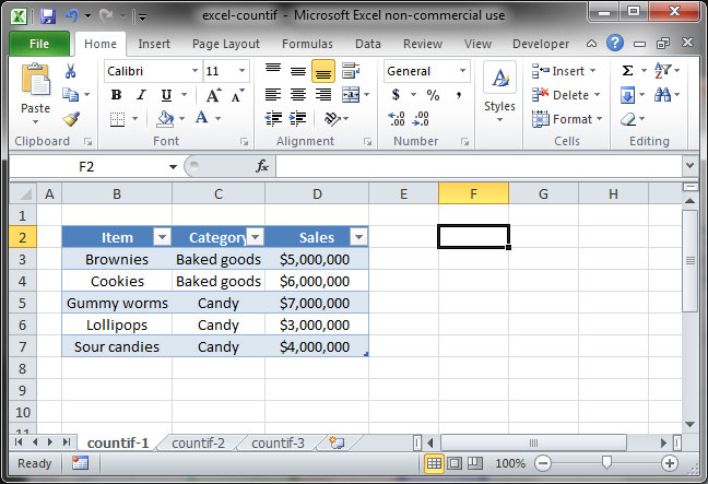
Take a look at the spreadsheet below, which lists SnackWorld sales by item and category.
Let's say we want to count up the number of items in the Baked Goods category. We could do this manually — which is fine for a small table like this one — but that becomes difficult when we have a table that contains a lot more data.
That's where COUNTIF comes in. It'll allow us to count the number of occurences of a particular phrase within a range.
COUNTIF in action
The formula for COUNTIF is as follows:
=COUNTIF(range, criteria)
Using the formula is simple: simply specify the range in which you would like to count values, and the criteria against which you'd like to count. Let's apply the formula to the sample spreadsheet shown above.
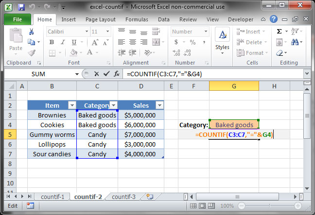
=COUNTIF(C3:C7, "="&G4)
In the above formula, we first specify the range C3:C7; Excel now knows that we want to count the number of occurences of a particular set of values within those cells. Then, we give it our condition: "="&G4. Excel looks in cell G4 and sees the value "Baked goods", so it knows we want to count the number of cells in our given range that contain that phrase. The answer in this case is 2.
Note that in this case, we're using the longform version of criteria — "="&G4. Like SUMIF, COUNTIF also has a shortcut when our criteria contains =: in the formula above, we could replace "="&G4 with a simple G4, like so:
=COUNTIF(C3:C7, G4)
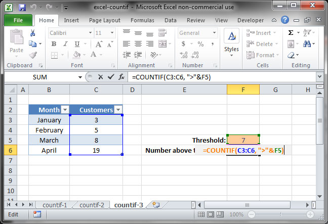
Let's take a look at another example in which we count the number of cells that contain values over a certain threshold:
=COUNTIF(C3:C6, ">"&F5)
In the above example, we count the number of months in which SnackWorld had more than 7 customers by counting occurences of a value greater than that found in cell F5 within the range C3:C6. In this case, the answer is 2. Try it yourself and take a look at how the answer changes as your threshold shifts up and down.
That's it! Now you know how to use the COUNTIF function in Excel.