Using Excel's MAX Formula

Oftentimes, you'll want to use Excel to find the maximum value in a range or series of numbers. For example, given a list of salespeople and corresponding dollar sales in any given month, you might want to find the maximum dollar sales to identify the highest-performing salesperson.

One way to accomplish this is by looking through your list of values and manually identifying the largest one. But that seems particularly time consuming and error-prone — especially if you're working with a big list. That's why Excel includes the MAX function. Using MAX, you can easily construct formulas that identify the largest value in a set. Keep reading to find out how.

A simple use of the MAX function

The MAX function is very simple to use; its basic syntax is as follows:

=MAX(number_or_range_1, number_or_range_2 (optional)...)

Note a couple of things here: first of all, the number_or_range arguments can contain either a number, like 4, or a range, like B4:B6. Second, you can insert as many number_or_range arguments as you want into the formula. Given these, Excel will output the largest value contained in either the numbers or ranges specified.

Let's take a look at a simple example to demonstrate this formula in action:

=MAX(4, 5, 6)
Output: 6

The above formula outputs the value 6, because 6 is the highest value supplied as an argument to the function.

Here's another example using a larger series of numbers:

=MAX(-7, 15, -100, 0, 3)
Output: 15

This formula outputs the value 15, because 15 is the highest value supplied to the function.

Using MAX with a range

Per the above, the MAX function can also be used with a range of values rather than a series of discrete inputs. Take a look at the following example, in which we use MAX to calculate the highest dollar sales by product category:

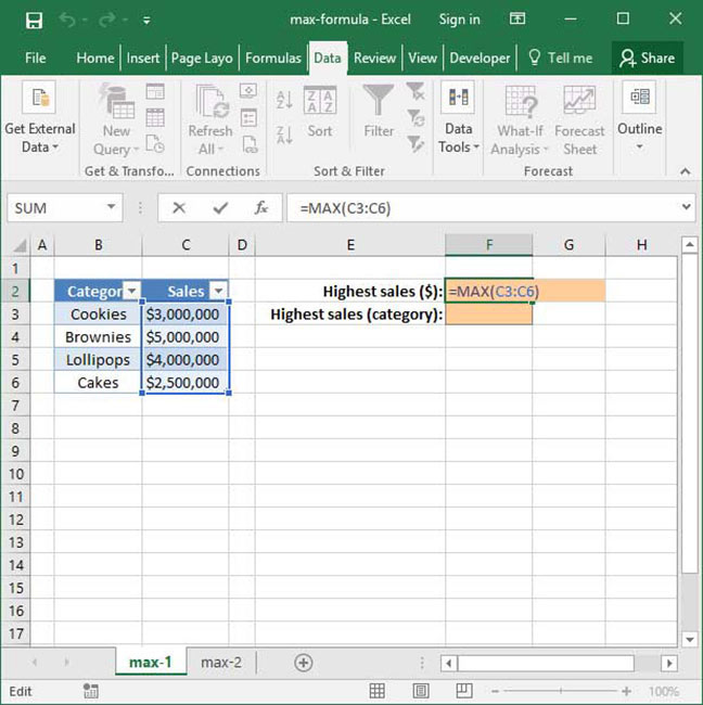
=MAX(C3:C6)
Output: $5,000,000

In the above example, we use MAX on the range of values representing dollar sales by category to extract the highest value — $5,000,000.

This is certainly useful, but what we really care about here is the name of the best-performing category — not necessarily the dollar value of sales within that category. Is there a way to extract just the name of the best-performing category using the MAX function?

The answer is yes — but to do so, we'll need to use a much more complicated function called INDEX MATCH. Take a look at the below example, in which we've combined MAX with INDEX MATCH to identify the best-performing category of the month:

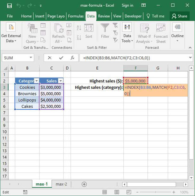
=INDEX(B3:B6, MATCH(F2, C3:C6, 0))
Output: "Brownies"

This may seem complicated, but if you'd like to learn more, head over to our INDEX MATCH tutorial. Once you've reviewed it and have a handle on how to use INDEX MATCH, come back here and see whether you can figure out why the above formula works like it does.

Other uses of MAX

Of course, MAX has many uses other than identifying the best-performing salespeople and categories. Here are some other ideas for how you can use MAX to make your life easier:

• Find the most recent day in a range of dates;
• Identify top-performing students by assignment;
• Find salespeople with the most sales in a given time range;
• Find the highest-recorded temperature in a given location; and
• Benchmark stock prices to maximum historical performance.

Questions on how to use MAX in a formula, or comments on this article? Sound off in the Comments section below!

Comments