VLOOKUP
VLOOKUP, one of Excel's most powerful functions, is used to look up data from a foreign table. Learn how to do a VLOOKUP in this handy tutorial!
In this lesson, we’re going to learn about one of Excel’s most common — and complex — functions: VLOOKUP. If you’ve been using Excel for a while, you’ve almost undoubtedly heard of VLOOKUP. It’s a common tool used in a huge number of spreadsheets around the world, and learning it is an important stepping stone to automating a lot of your day-to-day tasks in Excel.
Let’s start with an example of what the function can do. In short, VLOOKUP — which is short for “vertical lookup” — allows us to look up a given value from a vertically-oriented table of data. We’ve created an example workbook here so that you can see it in action. Our sheet lists 2016 SnackWorld sales numbers for a number of different product categories. We’ve created a VLOOKUP function that pulls the proper sales number if we enter the name of a given product category in this “Product” box up top. Check it out — when I enter “Cakes” into the box, our VLOOKUP function updates the “Sales” total to $1,646,500 — the sales total for the Cakes category. When I change the product category in our input box to Brownies, our Sales total changes accordingly.
You might be wondering why we wouldn’t just use Excel’s “Find” function if we wanted to find the Sales total for Cakes. We could pretty easily search for the word “Cakes” in our spreadsheet and find the sales total that way instead of writing a complicated formula.
The answer is two-fold:
First, we might be dealing with a mountain of data for which using Excel’s “Find” function would be too time-consuming. In this other sheet, for example, we’ve used the VLOOKUP function to pull in the categories of various products from an external table. There are a lot of orders, and looking up each of the product categories manually would have been way too time-consuming.
Second, the ability to dynamically update cells based on user input — like what we’ve done in our first sheet here — will become important down the line as we begin to develop more complex spreadsheets and models. We’ll investigate this further in later lessons.
Alright — so now that we know what VLOOKUP is, how do we use it? Getting a handle on this function is a bit complicated, but we’ll walk through it step by step to make it easy:
VLOOKUP takes four arguments: A value to look up, an array of cells in which to look up that value, a “column index number” that tells Excel how many columns into the array to look for a result, and a ‘range lookup’ argument that tells Excel whether to look for an exact match to your specified lookup term, or the closest match found in your lookup table. Let’s try it out using our sales data table from earlier. Recall that when using VLOOKUP, the table of data we use must be vertically-oriented — meaning that column headers appear along the top, and the value we want to look up appears along the side. We’ve also got to make sure that the value we want to look up — in this case, the name of a product — appears in the first column of the table in question.
Let’s get started. First, we’ll feed VLOOKUP a value to look up. In this case, let’s use the string, “Brownies”. Then, we’ll give it an array in which to look up our string. It’s important that when specifying the array here, we use our entire table rather than just the column in which our lookup value appears. In this case, our entire table spans from cells B2 to D17.
Next, we’ll give VLOOKUP a “column index number”. This number tells the function how many columns in to our data to look for a result. To use VLOOKUP, we literally have to count the number of columns of data we have.
In this case, we want to pull the number from the “Sales” column — which is one, two columns in to our data set. So, we’ll provide VLOOKUP with a column index number of 2.
Finally, we need to provide VLOOKUP with a ‘range lookup’ argument. This argument has to be either the word TRUE, or the word FALSE. If the ‘range lookup’ is TRUE, VLOOKUP will assume that your input array is sorted alphabetically — and will find the closest match to your specified lookup term. If ‘range lookup’ is FALSE, VLOOKUP won’t assume anything about the sorting of your input array — and it’ll only find an exact match with the term you specify.
When we use VLOOKUPs, we almost always set the ‘range lookup’ to FALSE. That way, we don’t have to worry about sorting our input table, and we know our VLOOKUP will only succeed if there is an exact match with our input term.
After pressing enter, our formula is complete. Note that VLOOKUP is pulling the correct value from the Sales column for the Brownies category!
Let’s make some changes in the formula to get an even better handle on how VLOOKUP works. First, we’ll change the lookup string to another product category, like “Cakes”. Note that when we change the string and press enter, our VLOOKUP formula updates its output to reflect the sales numbers for the Cakes category.
Second, we’ll try pulling lookup data from a different column. Let’s say that we wanted to pull data from our “Units sold” column rather than our “Sales total” column. To do so, we’d just have to update our column index number to three, since the “units sold” column is one, two, three columns into our input array. After making the update, our VLOOKUP automatically changes to reflect the proper number pulled from the “units sold” column.
Finally, we’ll wire our VLOOKUP function up to a dynamic input cell using cell references rather than manually coding our product name into the formula. Let’s enter a product name in cell G2, then replace the producy name in our VLOOKUP formula with a reference to cell G2. The output of our VLOOKUP formula automatically updates. And, like magic, our VLOOKUP will pull new data if we change the product name in cell G2. Note that we do need to provide VLOOKUP with a valid product name; an invalid product name will result in a formula error.
Now that our VLOOKUP is complete, I’ve got to warn you about one important caveat to this otherwise very useful function. Recall that in constructing our VLOOKUP, we had to manually count how many columns into our data table for the function to go to pull results. That’s fine and well, but it becomes a problem if we insert a new column into our data set. Check it out — when I put in a new column of data, our VLOOKUP no longer returns the proper results. That’s because it’s looking 3 columns into our data set for an answer — and the target column, “Units sold” is no longer 3 columns into our data set. After inserting this row, we’ll have to update our VLOOKUP function with a new ‘column index number’ to fix it.
Moral of the story: when using VLOOKUPs, always be careful when inserting columns into your data set, as it may have unforeseen consequences. That’s why I almost always recommend that Excel users replace their VLOOKUPs with a function called INDEX MATCH — which contains much of the same functionality, without this important drawback. We’ll explore INDEX MATCH in a later video in this module.
That’s it — you now know how to put together a VLOOKUP function in Excel! Take a look at the exercises bundled with this video to get more practice with this versatile function.
If you've spent time with Excel, you've probably heard of
In short,
That's a lot to take in, but things will become much clearer once we take a look at some examples below.
Defining the problem
Take a look at the simple spreadsheet below, which lists SnackWorld's January sales of various types of candy.
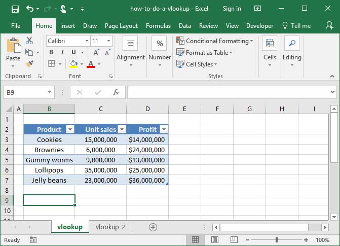
Let's say someone asked us how many Lollipops we sold in January. To answer their question, we'd have to open up the table, scan the rows until we find the word
That's easy to do when we have a small table like the one in the example above. But you can imagine it being very difficult if the table is large. It'd be a real pain to have to sift through hundreds of rows of data each time we want to look up the sales for a particular product.
That's where
Using VLOOKUP
Here's the syntax of the
=VLOOKUP (lookup_value ,table_array ,col_index_num ,range_lookup )
First,
Second, the function takes a
Third,
Finally,
We almost always use
Here's a complete example of the whole formula together:
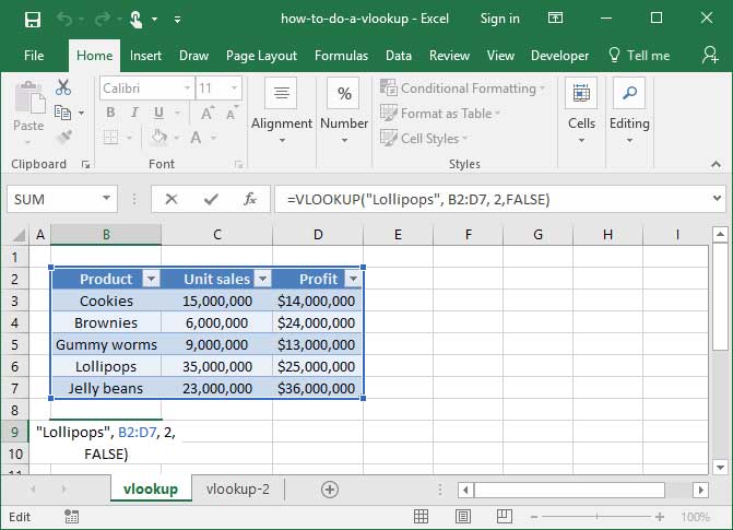
=VLOOKUP ("Lollipops" ,B2:D7 ,2 ,FALSE )
Output:35,000,000
What's happening here? First,
Next, it looks for the
Now, Excel knows that we want to pull some data from Row 6, since that's where it found the word
So, it follows the table across
Note that our
Another example
Let's check out another, slightly more complicated example of
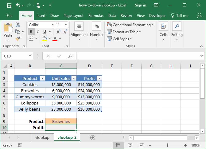
We want to write a formula in the empty grey box that will look up the
The answer: We'll use dynamic cell references within a
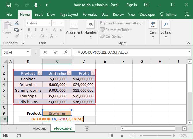
=VLOOKUP (C9 ,B2:D7 ,3 ,FALSE )
Output:$24,000,000
Let's break down what's happening here: First,
Now you can see how powerful