HLOOKUP tutorial

Want to perform a VLOOKUP, but not sure how to do so on a horizontal table? If you're struggling with this common Excel problem, then the HLOOKUP function is for you. It's just like a VLOOKUP, except that it performs lookups horizontally rather than vertically. Read on to find out how to use this handy formula.

Defining the problem

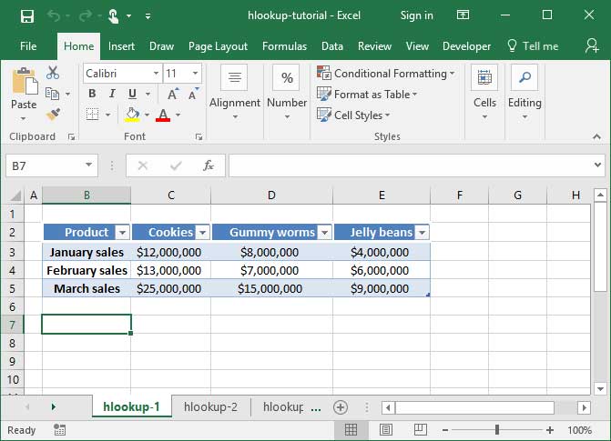
Let's say we have a table like the following, in which sales are listed horizontally by month and product.

If the table were oriented vertically, we would be able to look up monthly sales for a particular product by using a VLOOKUP. But since the table is oriented horizontally, we'll have to use an HLOOKUP instead. Let's take a look at how we do that.

Using the HLOOKUP function

The syntax of the HLOOKUP function is as follows:

=HLOOKUP(lookup_value, table_array, row_index_number, range_lookup (optional))

Much like VLOOKUP, HLOOKUP takes a lookup_value argument, which defines what the function will be searching for. It also takes a table_array argument, which specifies a table of data on which to search, and a range_lookup argument, which tells the function whether to search for a close match to our specified lookup term, or an exact match (we almost always use FALSE as our range_lookup argument to denote an exact match).

However, unlike VLOOKUP, HLOOKUP searches tables horizontally rather than vertically. Therefore, we need to provide a row_index_number rather than the column_index_number we're used to.

HLOOKUP in action

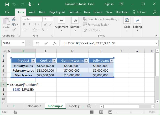
Let's take a look at the HLOOKUP formula used to solve the problem outlined above. In the below sheet, we'll perform an HLOOKUP to find Cookie sales in the month of February.

=HLOOKUP("Cookies", B2:E5, 3, FALSE)
Output: $13,000,000

What's happening in the above formula? First, Excel looks at our table_array argument, B2:E5, to get its bearings regarding the table we'd like for it to look up off of. Next, it examines our lookup_value argument, "Cookies", to determine which column on the table in question to look in. Finally, it sees our row_index_number argument, 3, and counts down three rows in the table in question.

Like with VLOOKUP, it's very important that the row from which our lookup_value is pulled is the first row in the table we specify in our table_array.

HLOOKUP with dynamic inputs

With HLOOKUP, we can also pull a lookup value from a dynamic input cell. You guessed it — just like with VLOOKUP! Let's check out an example in which we do just that:

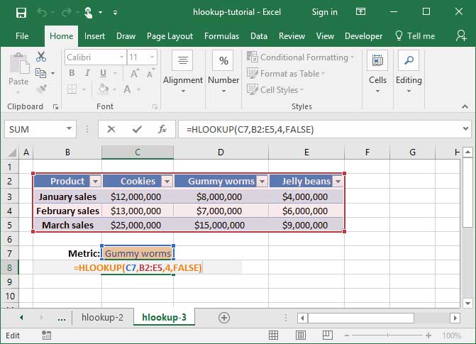
=HLOOKUP(C7, B2:E5, 4, FALSE)
Output: $15,000,000

In the above formula, we run an HLOOKUP on the range B2:E5. The lookup_value we provide references a cell, C7, which contains the phrase "Gummy worms" — so Excel scrolls over to the Gummy worms row to locate the data we're looking for. Finally, we've provided a row_index_number of 4, telling Excel that we want to scroll four rows down into the table in question. We arrive at the March sales row, in which we find the value $15,000,000.

HLOOKUP with wildcards

You can also use HLOOKUP with wildcards to match against a partial phrase or string. Take a look at our tutorial on wildcards in Excel for more information.

Comments