Using Excel's LEFT formula

Excel's LEFT function works almost exactly the same as RIGHT. This handy formula allows you to pull a specified number of characters from a string, starting with the leftmost characters and working right. Use it to extract data that lies on the left-hand side of a string, like a City in a City, State combination.

Let's take a look at how this function works.

Using the LEFT function

The syntax for the LEFT function is as follows:

=LEFT(text, num_characters (optional))

As you might guess, LEFT returns the leftmost num_characters characters of the text string you provide. Here are a couple of examples of LEFT in action:

=LEFT("San Francisco, CA", 3)
Output: "San"

=LEFT("Chicago, IL", 7)
Output: "Chicago"

=LEFT("Austin, USA", 6)
Output: "Austin"

Like RIGHT, LEFT's num_characters argument is technically optional. If you exclude it, LEFT will pull only the single leftmost character in the given text string, like so:

=LEFT("Austin, USA"
Output: "A"

Using LEFT with a variable num_characters argument

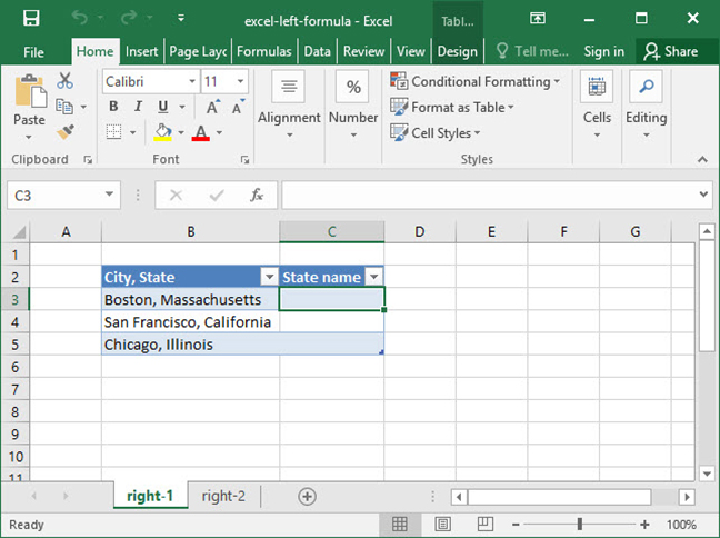
Like RIGHT, LEFT is also most commonly used with a variable num_characters argument to pull a particular substring based on a given delimiter. Take, for example, the following spreadsheet, in which we want to generate a formula to extract the name of a number of cities from City, State combinations:

In the above formula, we can't use a static num_characters, because the number of characters in each city name is variable. "Boston", for example, is a different length than "San Francisco".

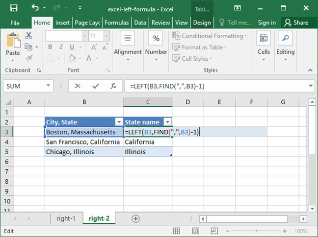
So, we construct a more elaborate formula using the FIND function to find the character that separates cities from states, ",", and run LEFT based off of that:

=LEFT(B3, FIND(",",B3)-1)
Output: "Boston"

What's happening here? First, Excel performs a FIND for the "," character, finding it at position 7 in the given string. We don't want to pull the 7 leftmost characters in the string "Boston, Massachusetts", because that would result in the string, "Boston," — with a comma at the end. So, we subtract 1 from the value given by our FIND function to get the number 6. We then use LEFT to take the leftmost 6 characters in the phrase, "Boston, Massachusetts", resulting in the string, "Boston".

Let's break things down step by step so we can get a better idea of what this function is doing:

=LEFT(B3, FIND(",",B3)-1)
Step 1: =LEFT(B3, 7-1)
Step 2: =LEFT(B3, 6)
Output: "Boston"

Note that this same formula also works when we translate it to other cells:

=LEFT(B4, FIND(",",B4)-1)
Step 1: =LEFT(B4, 14-1)
Step 2: =LEFT(B4, 13)
Output: "San Francisco"

Now that you have a good handle on Excel's LEFT formula, you can use it to extract data from strings that would otherwise be very difficult to handle. Enjoy!

Comments