How to Use Excel:
The Top 10 Things to Learn

Excel is one of the most powerful software tools in the world for collecting, analyzing, and summarizing data. But its incredible power comes at a cost: Excel is a massive program, and it can take beginners months or even years to master it. Many first-time Excel users don't take advantage of all of the program's functionality; we often find new learners manually entering data when they could be using formulas and functions to speed up and expedite their work.

With that in mind, we've compiled a list of the 10 most important places to start when you're learning how to use Excel.

The goal of this guide is to familiarize you with Excel's most useful functions — not to provide an in-depth overview of all of them. If you find yourself struggling to follow along, use the Further Reading section of each chapter for more detailed tutorials and additional examples.

Without further ado: here's our beginner's primer on how to use Excel — from worksheet basics to formulas and functions to Pivot Tables.

Cell and workbook basics

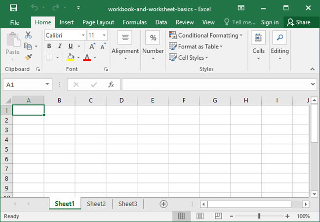
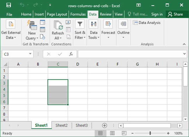
Before getting started with Excel, it's important to learn the program's basic structure so that you can navigate it effectively. Each Excel file is called a workbook — we often use the terms 'workbook' and 'file' interchangably when talking about Excel. Like many other programs, Excel allows you to save, open, and close workbooks from the File menu, which is located in the top left corner of the screen in the Ribbon, the menu of options along the top of an Excel document.

Pressing File leads us to the backstage view, an administrative area that gives us access to Excel's most important workbook-handling functions: Save, Open, Print, and Close:

Within each workbook, Excel contains multiple worksheets, which appear as tabs along the bottom of the screen. Worksheets are an easy way to contain multiple pages of data within one workbook in a logical manner. Generally, we place every individual calculation or table within its own worksheet to keep our data organized and easily accessible.

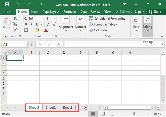
Each worksheet contains a grid of rows, columns, and cells. Rows appear along the side of the sheet, and are labeled using numbers starting with 1. Columns appear along the top of the sheet, and are labeled using letters starting with A. At the intersection of every row and column lies a cell, which is referred to by its address, which is a combination of its row number and cell letter. For example, the cell C5 lies at the intersection of row 5 and column C.

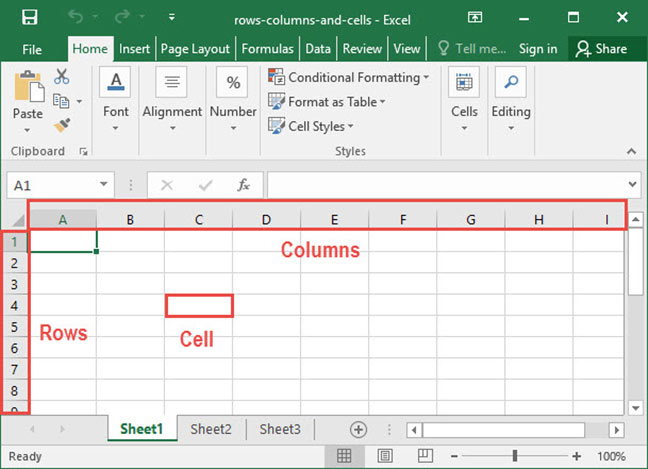
We can also refer to cells using ranges, which are series of contigous cells that lie next to each other. For example, the range between cells C3 and C6 can be selected all at once (see screenshot below). When we refer to a cell range, we put a colon (:) between the first and last cells within that range. Below, we've highlighted the range C3:C6:

When you select a cell and start typing, you can insert data into that cell. Data comes in a variety of formats, including numbers, letters, and equations. Any individual cell can contain any of the following types of data accepted by Excel:

• Numbers, which are numerical values like 5 or 78.34. Numbers can be used as part of calculations like addition, subtraction, and multiplication.
• Strings, which are bits of text like "Boston" or "SnackWorld". Strings can be manipulated in various ways, like finding pieces of text within them or chopping them in half.
• Dates, which represent days in our standard calendar, like 5/19/2019.
• Cell references, which point Excel to other cells in your workbook, like C9. We'll learn more about cell references further on in this tutorial.
• Functions, which are formulas that allow you to quickly and easily perform calculations that would be difficult to do by hand. These functions are often based on the contents of other cells within your workbook, and can output numbers, strings, or dates. And if you enter a function into Excel that doesn't make sense, it'll give you an error, like #N/A. Whenever you see an error like this, it means that there's a problem with your function and you need to revise it.

Those are the basics of workbooks and cells, but there's lots more to learn. Check out the more detailed articles below for further reading.

Further reading

• What is Excel? A beginner's overview
• Excel workbook and worksheet basics
• Working with rows, columns, and cells

Sorting and filtering data

One of the simplest and most immediately useful features of Excel is that it can sort and filter large sets of data incredibly quickly and easily. You can use this capability to alphabetize lists, order sales numbers by value, or screen lists down to a small subset of items based on criteria that you specify.

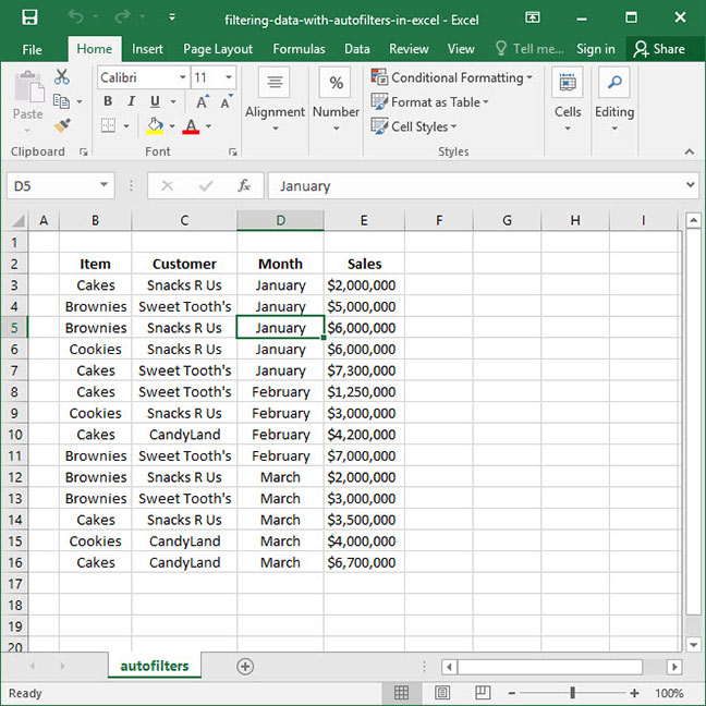
Take, for example, the below list, which contains a number of rows representing items sold by customer:

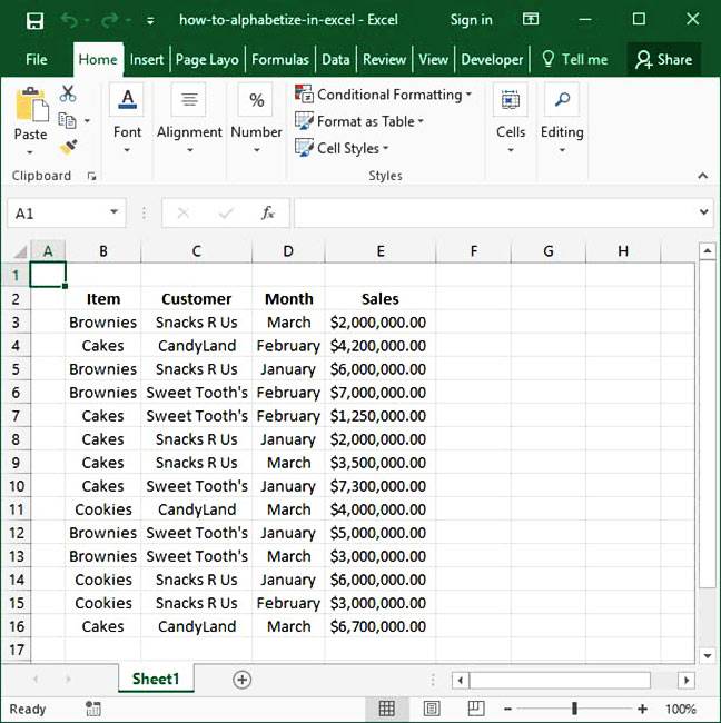
The above is a useful list, but it would be easier to read if we could sort by customer name to group all sales to the same customer together. To sort a list, position your cursor in the header cell of the column you'd like to sort, head to the Data tab on the Ribbon, and click the Quick sort button. In the below example, we've selected cell C2 to tell Excel that we want to sort by Customer name. Note our results after we press the Quick Sort button, which is highlited in yellow on the ribbon of the page below:

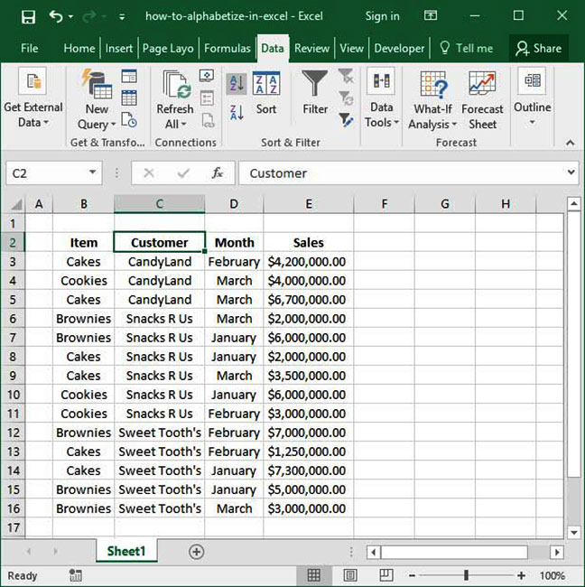
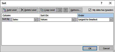
We can also sort data based on more advanced parameters by highlighting our entire data set and pressing the Sort button in the Data tab, highlighted in yellow below:

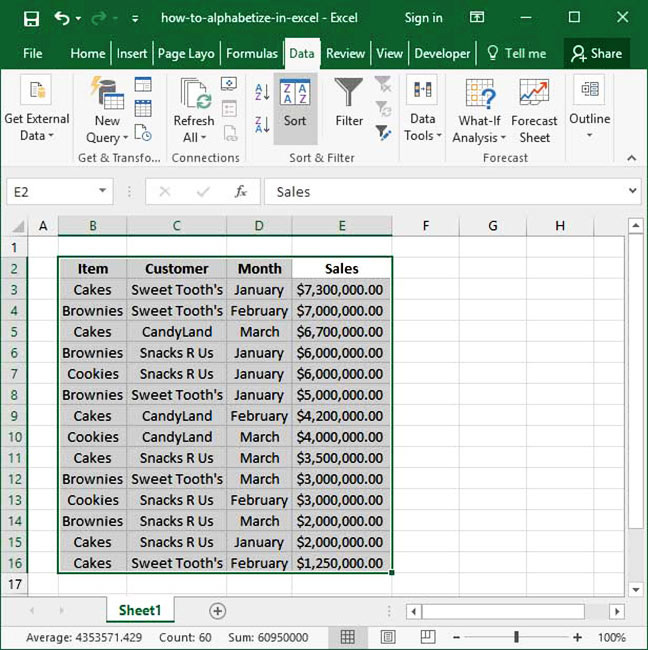
Pressing this button will open the Sort dialogue, which allows us to specify a set of more complicated sorting criteria — including sorting by multiple fields in a specified order.

In addition to sorting, we can also filter our data. Filtering means cutting down a large data set to a smaller subset of rows that satisfy certain specified criteria. To test filtering, we'll place our cursor within our data table, then head to the Data tab on the ribbon and hit the Filter option, highlighted in yellow below:

Notice that after filtering our data, small dropdown arrows appear next to the headings of each of our columns. We can click these arrows to open up the Filter Dialogue, which allows us to filter our data set so that it shows only certain rows. Below, we've used the Filter Dialogue to select only rows for which the Month is equal to February.

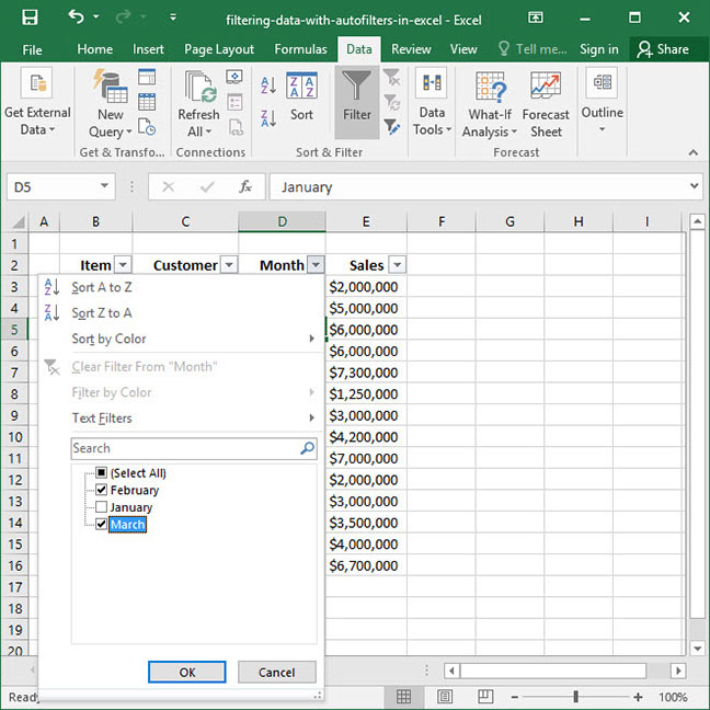
When we press the OK button, our data set will be trimmed down: now, only February rows are shown.

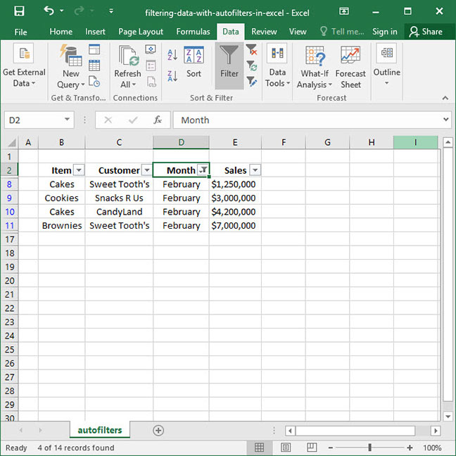
The beauty of filtering is that no rows have actually been deleted; our entire original data set is preserved. We've just temporarily filtered out rows in which the Month is equal to anything other than February. Notice the blue row labels on the left-hand side of the screen — those indicate that our data has been filtered.

Now that you know how to use basic sorting and filtering, check out our more in-depth articles below. They'll show you how to perform advanced custom sorts and add multiple filters based on dates, values, and text.

Further reading

• How to alphabetize in Excel: A complete guide to sorting
• How to filter data with autofilters in Excel

How formulas work

Formulas are the backbone of most advanced calculations within Excel. Think of a formula as an equation — it's a series of steps that lead to a final output. You can tell Excel that you're entering a formula in Excel by starting your input with the equals sign (=). For example, try entering the following into a cell:

=5+4
Output: 9

Since Excel sees the = sign at the beginning of the line, it realizes that it's being given a formula to calculate. It then sees 5+4 and adds the two numbers together, outputting a final value of 9.

Formulas often contain more than just numbers and operators like the + sign. They can also contain one or more functions. Think of a function as a machine that helps you quickly and easily make calculations that would be difficult to perform by hand. Each function is like a recipe: it takes in a list of ingredients, and the recipe spits out something totally new — and, in most cases, more useful than what you put in. Each function is made up of three parts:

• First, a function name, which describes what the function does — like the name of a recipe. Function names are built into Excel. For example, there is a SUM function that adds together a series of values, and a AVERAGE function that averages together multiple values. We'll explore the various functions available to you throughout these tutorials.
• Second, arguments, which combine within the function to output something bigger — like the ingredients of a recipe. For example, if we wanted to take the AVERAGE of 4 and 6, the arguments to the function would be the numbers four and six. In a function, arguments are separated by commas within parentheses.
• Third, output, which is what comes out of the function when it's finished calculating — like the final product of a cooked recipe. For example, if we took the AVERAGE of 4 and 6, the output would be 5.

Take a look at the examples of completed formulae below. Can you identify the function names, arguments, and output?

=AVERAGE(4, 6)
Output: 5

=MAX(4, 6, 2, 34)
Output: 34

Within formulae, we can also nest functions. Nesting functions means using the output of one function as the argument for another. For example, if we wanted to AVERAGE the numbers 4 and 6 and add the resulting value to the number 10 using SUM, we could do so by nesting functions like so:

=SUM(AVERAGE(4,6),10)

Notice that we've included the AVERAGE function within the SUM function, effectively nesting the two functions together. Whenever Excel encounters nested functions like these, it evaluates them starting on the inside and working out. For the sake of simplicity, throughout these tutorials, we'll evaluate nested functions step-by-step just like Excel does to show you every stage of the process, like so:

=SUM(AVERAGE(4,6),10)
Step 1: =SUM(6,10)
Output: 16

Nesting isn't just limited to two layers — you can nest as many functions within each other as you'd like. Take a look at the following formula — which we haven't broken down step-by-step — and see if you can figure out why it outputs what it does.

=SUM(SUM(AVERAGE(1, 3), AVERAGE(5, 7)), SUM(12, 10))
Step 1: =SUM(SUM(2, 6), SUM(12, 10))
Step 2: =SUM(8, 22)
Output: 30

You now know the basics of how to use formulas and nested functions in Excel. Check out the tutorials below for more detailed information!

Further reading

• What is a function in Excel?
• Excel nested functions

Cell references

Excel really starts to get insteresting when you start using cell references. Cell references are parts of a formula that connect to another cell or cell range within your worksheet.

Take a look at the following formula, which contains the most basic type of cell reference:

=C4

In this piece of code, we're telling Excel to go to cell C4, evaluate it, and return whatever value it contains. Likewise, we could ask Excel to look at cell E6 and pull its value like so:

=E6

Cell references are useful because they can be included within functions. This enables you to perform complex calculations based on sets of cells that would otherwise be difficult to perform manually. For example, take the following SUM function:

=SUM(C3:C7)

This function will automatically SUM up all values in the entire range C3:C7 — in other words, cells C3, C4, C5, C6, and C7.

By default, cell references are relative. This means that they will change as we copy and paste them from cell to cell. Let's take a look at an example to clarify what this means.

The following spreadsheet contains sales data for three product categories (Cookies, Brownies, and Gummy Worms), as well as a blank Total row. We've inserted a SUM formula in the Total row to calculate total Cookies sales by summing cells C4:C6:

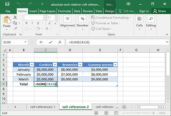
=SUM(C4:C6)
Output: $16,000,000

Our total is set for Cookies, but we'd like to it to display for the other product categories as well. Let's copy the formula in cell C7 by pressing Ctrl + C on Windows or ⌘ + C on a Mac. Then, we'll click and drag to select cells D7 and E7 and paste our formula using Ctrl + V on Windows or ⌘ + V on a Mac.

Notice what happens to the formula in cell D7 — it changes! Our formula now references the cell range D4:D6 instead of C4:C6. This is the magic of relative cell references. As we copy and paste formulas from cell to cell, our references change to accomodate.

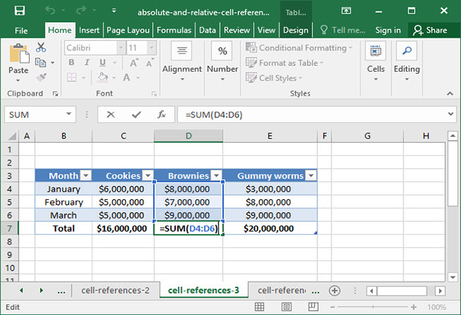
=SUM(D4:D6)
Output: $24,000,000

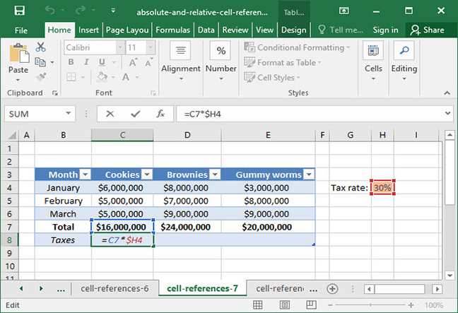
Relative cell references are convenient, but there are some times during which we don't want our cell references to shift when we copy and paste. Consider the following sheet, in which we've created a static value in cell H4 to represent a tax amount taken off of our total sales:

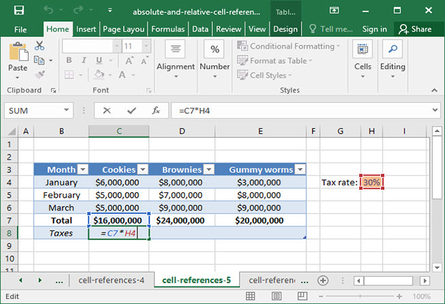
=C7*H4
Output: $4,800,000

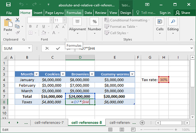
Our formula works in cell C8, but when we copy and paste it to the right, our relative cell references change and our formula breaks:

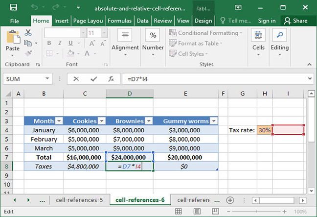
=D7*I4
Output: 0

Fortunately, there's a good solution to this problem: absolute cell references. Absolute cell references allow us to lock the row or column of a reference — or both! — so that they do not change when we copy and paste from one cell to another.

The $ symbol indicates an absolute cell reference. It can be used before the column letter, the row number, or both, and indicates that the given column letter or row number should not be changed when copying and pasting from cell to cell.

Here's an updated version of our formula, with an absolute reference used to lock the column letter on the reference to our tax rate cell, $H4:

=C7*$H4
Output: $4,800,000

Notice what happens when we copy and paste this formula to the right. Our $H4 reference doesn't change, because the column letter is locked. Our formula now works for all cells into which we're pasting it!

=D7*$H4
Output: $4,800,000

When working with absolute and relative cell references, it's important to remember that you can use them on the row, column, or both. Here's a handy table to help understand what that $ symbol means when it appears:

Remember, rows and columns in a cell range can also be locked. For example, the range $A1:$B8 will have its columns locked as it is copied and pasted. The range A$1:B$8 will lock its rows.

Those are the basics of cell references — both relative and absolute. Check out the article below for more detailed information.

Further reading

• Absolute and relative cell references

Mathematical functions

Now that we've covered the basics of Excel, it's time to get into the program's more advanced features — starting with mathematical functions themselves. Excel has hundreds of functions available for use, and it would be impossible to cover all of them in this short tutorial. So, to start, we'll provide a brief overview of some of Excel's most common mathematical functions.

SUM

SUM is one of Excel's simplest — and most-used — mathematical functions. It can take as many arguments as you want to give it, in the form of numbers, cell references, or cell ranges. Given these arguments as inputs, it outputs the SUM of all values provided — including each individual cell within a cell range.

Here's a basic use of the SUM function, in which we add up a series of manually-entered numbers:

=SUM(3, 7)
Output: 10

Here's a slightly more complicated use of the SUM function, in which we add up a series of individual cells by specifying them as unique arguments to the function:

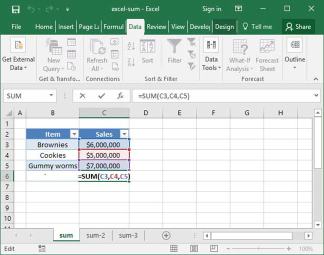
=SUM(C3, C4, C5)
Output: $18,000,000

And, finally, here's a better use of the SUM function, in which we use a cell range to add up the values in a series of contiguous cells:

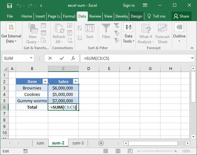
=SUM(C3:C5)
Output: $18,000,000

Check out our detailed SUM tutorial for even more details and information.

AVERAGE

The AVERAGE function works much like the SUM function: it takes as arguments a list of numbers or cell ranges. Unlike SUM it outputs the AVERAGE of the values provided.

Here's a basic use of AVERAGE in action:

=AVERAGE(10, 20)
Output: 15

And here's AVERAGE used with a cell range:

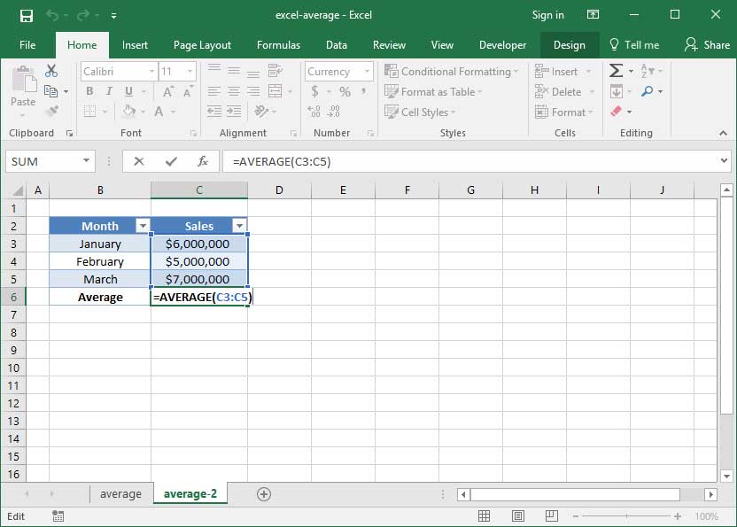
=AVERAGE(C3:C5)
Output: $6,000,000

Head over to our overview of the AVERAGE function for more info.

MAX

The MAX function starts to get a little more complicated: given input arguments of numbers, cell references, or cell ranges, MAX finds the maximum individual value provided and outputs it. MAX is particularly useful when working with large quantities of data to determine high values within a set — like students' highest score on a test or a daily high stock price.

Take a look at the following formula, in which we've used MAX to find the maximum value within a series of individual numbers:

=MAX(4, 5, 6)
Output: 6

Of course, like SUM and AVERAGE, MAX is most useful when applied to large ranges of cells. Consider the following example, in which a SnackWorld analyst uses MAX to find the highest dollar sales value out of a set of product categories for a given month:

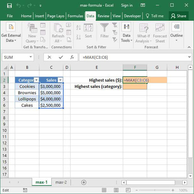
=MAX(C3:C6)
Output: $5,000,000

MAX has many applications, and as you get more and more comfortable with Excel, you're sure to find multiple uses for it within your spreadsheets. You can also use the closely-related MIN formula to find minimum values within a set. Check our our MAX and MIN tutorials for more.

COUNT

COUNT is another frequently-used function in Excel. Given a cell range or set of values, it counts the instances in which a number appears in the given range. Consider the following example:

=COUNT(5, 9, 10)
Output: 3

The above formula outputs 3, because there are three instances of numbers provided as arguments. A COUNT function provided with non-numerical inputs would not count them — it would only include the count of numbers provided as arguments:

=COUNT(5, "Seven", 10, #N/A, 45)
Output: 3

COUNT can also be used on a range of values like so:

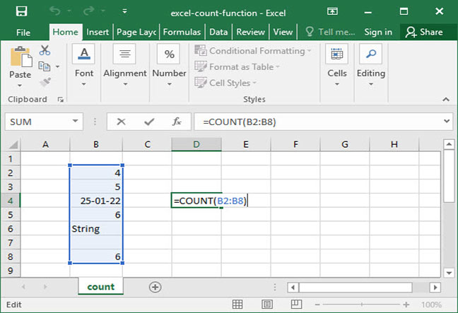
=COUNT(B2:B8)
Output: 5

How is this useful in practice? Use the COUNT function in your sheets to count data points, like number of test scores, number of items sold in a given period of time, and more. COUNT also has a sister function called COUNTA, which includes cells that contain text in its totals. Stop by our COUNT and COUNTA tutorial pages for more info.

Further reading

• Excel's SUM function
• AVERAGE formula in Excel
• Using Excel's MAX Formula
• Minimum Values in Excel Using MIN
• How To Use Excel's COUNT Function
• Using Excel's COUNTA Function

Lookup functions

Now that we've got a handle on some of Excel's basic mathematical functions, it's time to move on to a more complicated class of tools: lookups. Lookup functions allow us to look up a given value on a table with multiple rows and columns dynamically. That's quite a mouthful, so let's take a look at a real-world example to give you an idea what we mean.

Take a look at the below spreadsheet, which lists SnackWorld unit sales and profit for various item categories in a given month.

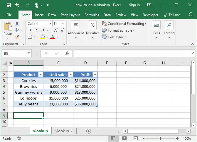
Let's say that a SnackWorld analyst wants to pull the Unit Sales number for the Lollipops category. She could just look it up on the table — but manually looking it up becomes infeasible if the table is too large — for example, if it contains hundreds or thousands of rows and columns. It's also time-consuming. What if we could create a tool in which we enter a category name, and the Unit Sales number for that category is automatically pulled from our input table?

VLOOKUP

We can accomplish the above using the VLOOKUP function. VLOOKUP takes a table and a lookup value as inputs, browses the given table for the lookup value in question, and finds whatever sits in a corresponding column number specified. Here's how it works:

=VLOOKUP(lookup_value, table_array, col_index_num)

Given a set table_array, VLOOKUP finds the given lookup_value within that array, then moves over col_index_num columns to pull the corresponding data point. Take a look at the following use of VLOOKUP in action, in which we use the formula to pull the unit sales numbers for Lollipops:

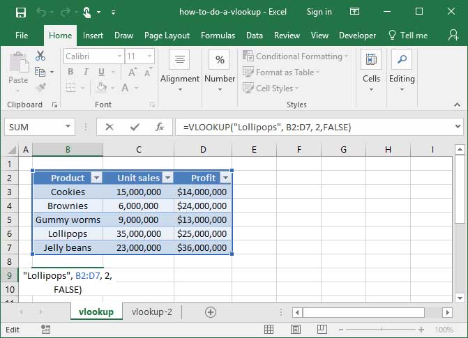
=VLOOKUP("Lollipops", B2:D7, 2)
Output: 35,000,000

In the example above, we provide VLOOKUP with a lookup value, "Lollipops", and a table to look in B2:D7. We also tell it that in the table specified, we want it to look 2 columns in for the data point, which corresponds to the Unit Sales column. When VLOOKUP finds the "Lollipops" value in our table B2:D7, it moves over 2 columns and pulls our unit sales number: 25,000,000. We've just successfully created a simple lookup formula!

How is this useful in practice? VLOOKUP can be used with cell references to create a dynamic data-pulling tool very quickly and easily. Take a look at the following example, in which we've used cells C9 and C10 to create dynamic input and output fields for a formula to pull profitability numbers:

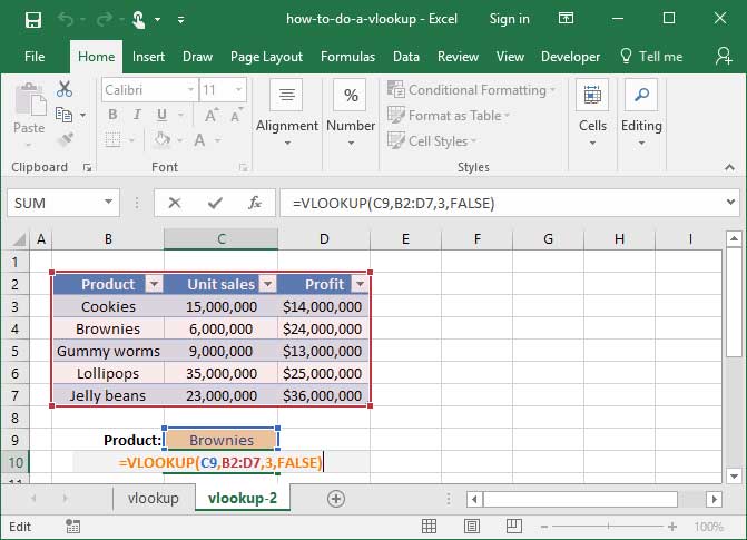
=VLOOKUP(C9, B2:D7, 3)
Output: $24,000,000

Notice that our VLOOKUP formula now references cell C9 instead of a hard-coded value like "Lollipops". And when we change the text in C9 to another category name on our table, the formula in C10 automatically updates by pulling profitability numbers for the given category. Like magic, we've created a quick tool to pull data based on simple user inputs — all with one simple VLOOKUP formula!

Check out our in-depth VLOOKUP tutorial for more info on this powerful function.

INDEX MATCH

Once you've mastered VLOOKUP, it's time to move on to an even more powerful lookup formula: INDEX MATCH. INDEX MATCH isn't actually a single function, but rather a combination of two separate Excel functions: INDEX and MATCH. We use it in place of VLOOKUP for almost all of our lookups, because it confers several important advantages:

• Counting isn't necessary. VLOOKUP forces you to count columns, providing it with a col_index_num to indicate which column to pull data from. INDEX MATCH allows you to skip this step, instead selecting the column in question directly.
• Inserting columns is easy. Since VLOOKUP uses a col_index_num for its lookup, inserting columns into your lookup table can often break your formulas. INDEX MATCH prevents these problems by eliminating the col_index_num argument.
• Backwards lookups are possible. INDEX MATCH allows you to look up values that are to the left of your item or category list, rather than only those that are to the right.
• Even more functionality. INDEX MATCH allows you to take advantage of a plethora of more advanced functionality — including both vertical and horizontal lookups; two-dimensional lookups; and lookups with more than one criteria.

Covering how INDEX MATCH works is beyond the scope of this tutorial, but check out our complete guide to INDEX MATCH for more information and a full explanation.

Further reading

• How to do a VLOOKUP
• Using INDEX MATCH
• Using INDEX MATCH MATCH (look up in two dimensions)
• INDEX MATCH with multiple criteria

Logical functions

Logical functions are some of the most advanced formulas you can create in Excel. They allow us to tell Excel to choose one of various possible outputs depending on a condition that we specify. This functionality becomes incredibly useful when you want Excel to make decisions for you: for example, marking a test score as "Passing" if it is over 70%; marking a salesperson's quota as "met" if she has exceeded $20M in monthly sales; or marking a stock as "High-priority" if its price drops below a certain limit.

IF statements

IF statements are the foundation of logical functions in Excel. IF statements look like this:

=IF(logical_expression, value_if_true, value_if_false)

When an IF statement runs, it first takes a look at the logical_expression provided by the user. If the logical_expression is a TRUE statement, the IF statement outputs value_if_true; otherwise, it outputs value_if_false.

Let's take a look at a very basic IF statement as a practical example:

=IF(7<3, "Correct answer!", "Incorrect answer")
Output: "Incorrect answer"

In the formula above, IF first evaluates its logical_expression, 7<3. Since this expression is FALSE, Excel ignores the value_if_true argument and instead outputs the value_if_false argument, "Incorrect answer".

Of course, the above example isn't particularly useful, because we don't need a complicated formula to tell us that 7 is not equal to 3. But IF becomes significantly more useful when we combine it with other functions — for example, SUM.

In the following example, we use IF statements to dynamically provide output based on whether a salesperson met her sales quota for the first quarter of the year. The salesperson's monthly sales are listed in a table; we nest a SUM function inside an IF statement to total up the sales and compare it to a quota, which we've included in the formula via a cell reference.

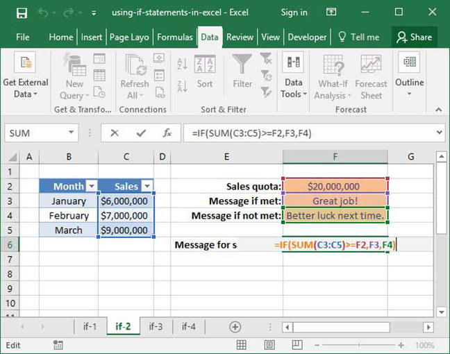
=IF(SUM(C3:C5)>=F2, F3, F4)
Step 1: =IF($22,000,000>=$20,000,000, F3, F4)
Step 2: =IF(TRUE, F3, F4)
Output: Great job!

Let's break down what's happening in the above formula. First, our IF statement evaluates its logical_expression, which asks whether the SUM of cells C3:C5 is greater than or equal to the value in cell F2. If it is, the sales quota is met and the formula outputs its value_if_true, which is set as a cell reference to the text in cell F3. If not, the sales quota is not met and the formula outputs its value_if_false, which is set as a cell reference to the text in cell F4. In this case, our sales quota is met, and the formula outputs a message of congratulations: "Great job!". But try lowering the values in cells C3:C5 so that their sum is below $20,000,000. You'll see that our message changes dynamically once our salesperson falls below quota.

Those are the basics of IF statements, but you can do much more with them than just compare whether two values are equal to each other, or whether one is greater than the other. Check out the following list of logical operators in Excel for a full overview of how IF can be used to compare values or strings:

For more information, stop on by our tutorial on IF statements.

SUMIF

Once you've got a handle on the IF statement, it's time to move on to an even more useful Excel feature: SUMIF. This handy function allows us to take the SUM of every number in a range of values, provided that certain external criteria for those values are met.

Let's take a look at a basic example of SUMIF in action to demonstrate. Consider the following spreadsheet, which lists SnackWorld's monthly sales by item type and product category.

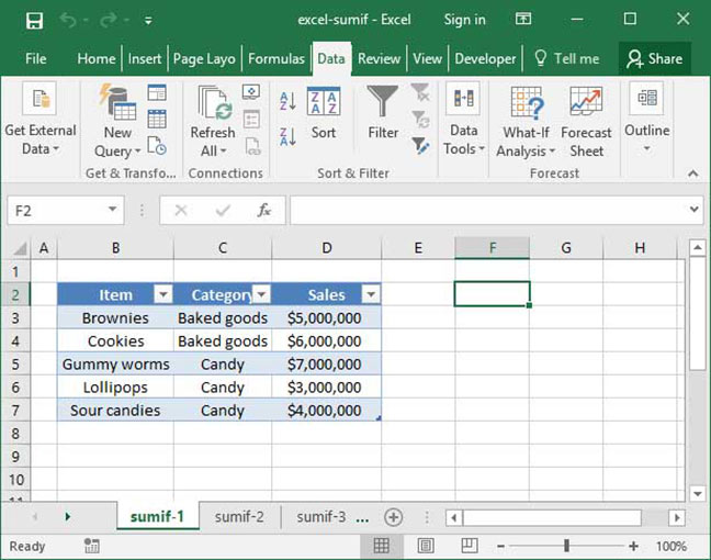
We already know how to use VLOOKUP and INDEX MATCH to dynamically pull the sales numbers for any individual Item. But what if we wanted to SUM up sales for every item within a given Category?

We can do this using the SUMIF function. Take a look at its syntax below:

=SUMIF(range, criteria, sum_range (optional))

Given an input range of data points and a set criteria that we want those data points to fulfill, SUMIF will take the SUM of all numbers within a separately-provided sum_range. Here's a practical example of SUMIF used to solve our category problem above:

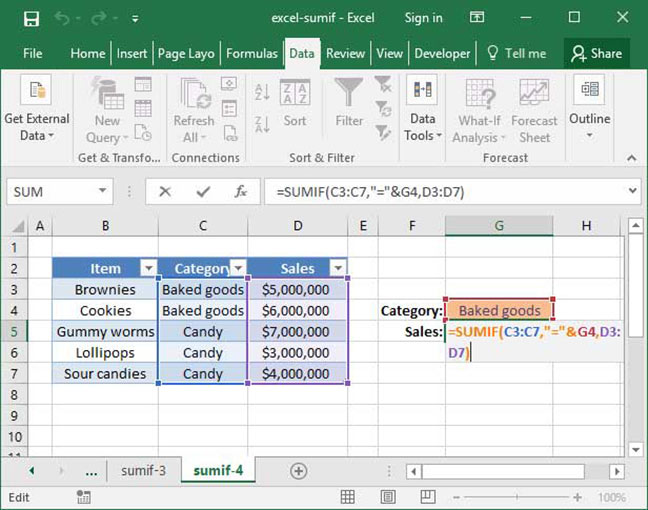
=SUMIF(C3:C7,"="&G4,D3:D7)
Output: $11,000,000

In the above example, SUMIF takes a look at the range C3:C7 and evaluates each cell in that range based on its provided criteria: the value in the given cell is equal to the value in cell G4. Note the syntax we've used to tell Excel that we want to evaluate equality to cell G4: The = sign, in quotes, the ampersand (&), and then a reference to cell G4. This syntax might be confusing at first, but it's just how SUMIF works; note that we can replace that = sign with any other logical operator, like <= or <>.

After examining each cell in the range C3:C7, Excel adds the corresponding value in the range D3:D7 to a SUM total if and only if our criteria is true — in this case, if the Category is equal to the value in cell G4, "Baked Goods". In this case, our final output is $11,000,000, because there were $11,000,000 total sales of Baked Goods in the data set provided.

The best part about this formula is that it's dynamic. Try changing the string in cell G4 from Baked Goods to Candy and watch as our category sales calculation automatically updates.

The above may take a little time to digest, but walk through it a couple times and you'll get a handle on how SUMIF works. If you're still having trouble, take a look at our in-depth SUMIF tutorial for more details and examples.

Once you've mastered SUMIF, it's also worth checking out our overview of SUMIFS, which is SUMIF's big brother. SUMIFS allows you to conditionally SUM values in a row based on multiple criteria rather than just a single criteria.

It's also worth noting that SUM isn't the only function that has a conditional formula. COUNTIF works much the same way, but it COUNTs rows instead of SUMming them.

Further reading

• The TRUE and FALSE Excel functions
• Using IF statements in Excel
• Excel's SUMIF function
• Excel SUMIF with multiple criteria: SUMIFS
• Excel's COUNTIF function

Creating charts

Formulas and numbers aren't all that Excel has to offer. In addition to displaying data numerically, it's also excellent at displaying data visually using charts and graphs. In this section, we'll give you a brief overview of Excel's charting capabilities, and show you how to generate graphs based off of your data.

The most important first step to creating a chart is preparing your data. To generate a chart, you'll need to create a data summary table that shows the exact data points that you'd like to appear on your chart. Oftentimes, we create summary table for use with charts and graphs by leveraging the Excel functions we discussed above, including lookups, SUMIF, and COUNTIF. In the example below, we've consolidated a list of SnackWorld sales by category and month.

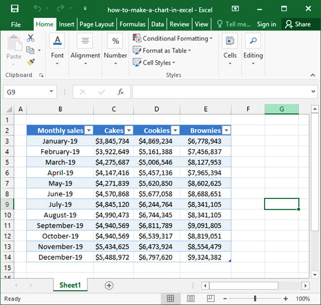
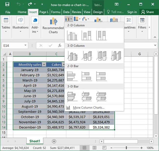
Once your data is ready for charting, select your entire table by clicking and dragging your mouse, or using hotkeys (Ctrl + A using Windows or ⌘ + A on a Mac). Then, navigate to the Insert tab on the Ribbon, hit the Charts button, and select the type of chart you would like to create. In our example, we'll create a Clustered Column chart from our data.

Our chart is created! With just a few simple clicks, we've taken a data summary table and made it visually clear and accessible for our users.

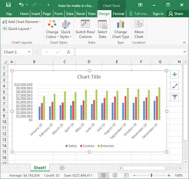
There are many different chart types available in Excel, so it's important to think carefully about which visual will most clearly communicate your data. In the example below, we've used the same data to create a Stacked Column chart, which gives us a more useful look at total sales by month segmented by product category.

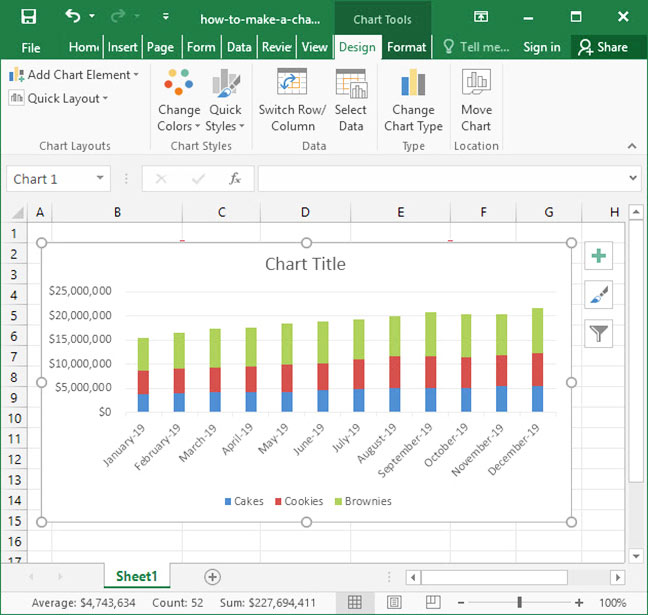
Of course, the chart above is lacking some crucial details — for example, it doesn't have a title, so we have no idea what year our data comes from (or, for that matter, what company's sales data it represents). Once you've created your chart, ensure that your users have all the data they need by adding a title, axis labels, and other formatting, like a legend and data labels. All of these options are available when you select your chart and go to the Layout tab on the Ribbon:

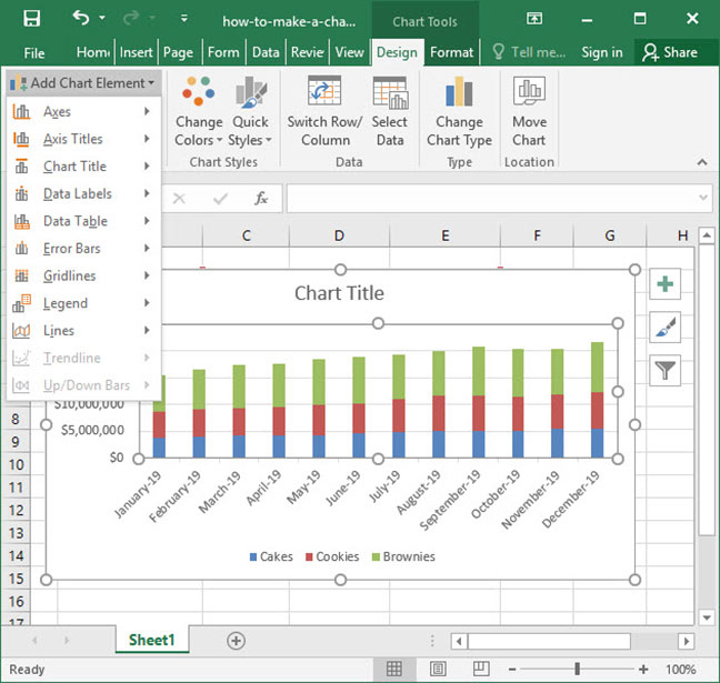
There are many complex charting options in Excel — including advanced features like manually-set axis labels, statistical analysis, and customized styling. Play around with the options in the Layout, Design, and Format tabs on the ribbon to familiarize yourself with the full range of Excel's capabilities. Or, check out our in-depth article on charting for more information.

Further reading

• How to make a chart in Excel

Pivot Tables

Once you've mastered Excel's basic formulas — like SUM, SUMIF, IF statements, and VLOOKUPs — you should be able to perform some fairly complex analysis on your spreadsheets given enough time. But what if you need to perform calculations quickly and accurately under tight deadlines? Oftentimes, writing formulas it too time-intensive and error-prone for real business applications, particularly when faced with time constraints.

Fortunately, there's an easy alternative to complex formulas: Pivot Tables. Pivot Tables are a tool built into Excel that allows you to analyze large amounts of data quickly and accurately. Let's take a look at a Pivot Table in action to explain the concept.

The spreadsheet below contains sales data for a number of SnackWorld orders in the first quarter of the year 2019.

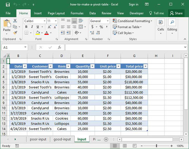
The data is in what we call flat file format, which means that it is broken down to its most granular level: each individual order is on its own line; all relevant information (including the customer name, order date, quantity ordered, item, and total price) is broken out in each row; and each column heading represents a distinct type of data (like Customer or Item) rather than a data point (like January 2019 or February 2019). Making sure that our data is properly structured in flat file format is a critical first step in building a Pivot Table. For more information and specifics on flat file format, be sure to check out our article on how to make a Pivot Table.

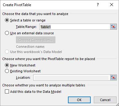
Once we've got our data in order, we can make our Pivot Table. Start by selecting any cell within the input data table; then, head to the Insert tab on the Ribbon and select the PivotTable option:

A Create PivotTable dialogue will appear. We can change some of these options when we get to more advanced Pivot Table training down the line, but for now feel free to leave everything as-is and click the OK button:

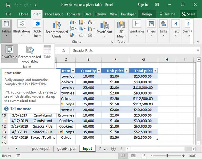
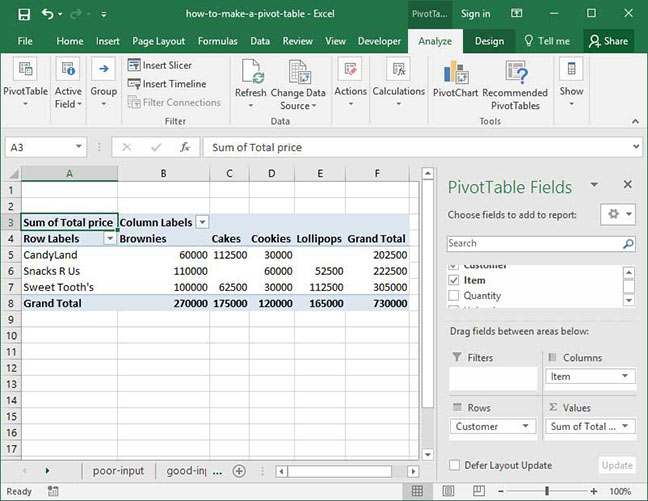
A new sheet will appear that contains our Pivot Table. Notice that Excel has inserted a blank Pivot Table graphic on the left-hand side of the screen, and opened a new PivotTable Field List dialogue on the right:

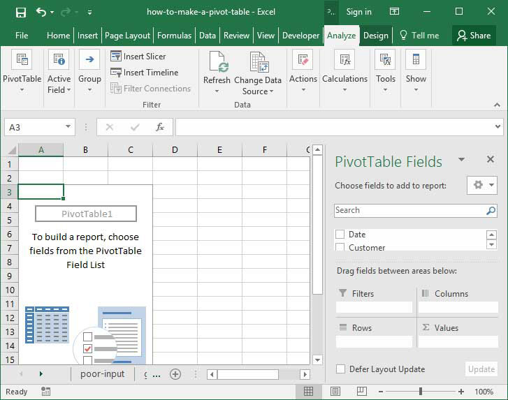
The PivotTable Field List contains a listing of all of the column headings within the data table we used as an input. We can add any of these column headings to the Report Filter, Column Labels, Row Labels, and Values sections below to generate different types of Pivot Table reports that segment our data different ways. Specifically:

• Report Filter allows us to filter our output based on the values in one or more fields.
• Column labels lets us summarize by a particular field across the top of the screen (columns).
• Row Labels lets us summarize by a particular field down the side of the screen (rows).
• Values Specifies the column data that we'd like to summarize — for example, Total price.

That's all a lot to keep track of — so let's take a look at a real-life example to get a better handle on what this all means. Suppose that a SnackWorld analyst wants to summarize total sales by customer over the entire period contained within our data table. She could do so by dragging the Customer column to the Row Labels section — to indicate that we want each row of our Pivot Table to represent a unique customer — and the Total Price column to the Values section — to indicate that we want to sum up Total Price by customer. Move the field names around to different sections of the Pivot Table by clicking and dragging with your mouse.

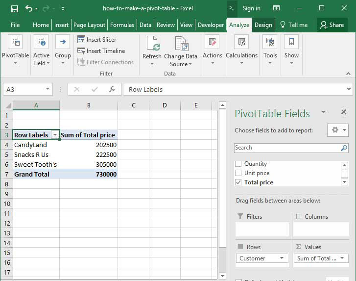
Without any formulas or functions, Excel has automatically added up the Total Price column for each of our customers. We've created an accurate summary table quickly and easily with minimal effort based on a large input data set — that's the magic of Pivot Tables!

There are lots more things we can do with Pivot Tables by moving our columns between the four boxes at the bottom of the screen. For example, by dragging the Quantity column into the Values section alongside Total Price, we can sum both fields at once, segmented by customer. This view shows both total sales dollars and total quantity of goods ordered by customer:

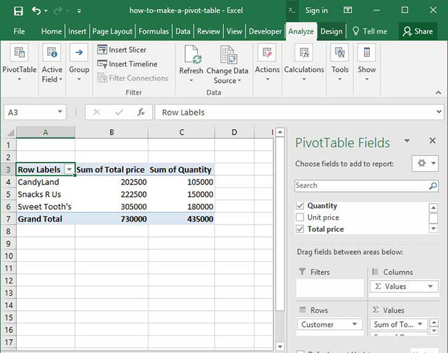
We can also drag another field — like Item — to the Column Labels section of the report to create a two-dimensional summary breaking out total sales by customer and item:

Or, we can drag a field to the Report Filter section to filter our output table based on one or more criteria that we specify. In the following example, we've dragged the Item column to the Report Filter box to open up a dialogue that allows us to filter our output based on item type.

The power of Pivot Tables is practically limitless — they can be used in a massive variety of situations to segment and summarize data. They're particularly valuable when calculating a SUM, COUNT, or AVERAGE across a large data set. For more detailed information about how to set up and use Pivot Tables, be sure to check out our in-depth explanation of Pivot Table features.

Further reading

• What is a Pivot Table?
• How to make a Pivot Table

Advanced formatting

Now that you've got a handle on data manipulation in Excel, it's time to learn some advanced formatting techniques to polish your spreadsheets — making them both beautiful to look at and easy to interpret.

The most useful of these features is called Conditional Formatting. It's an Excel tool that allows you to format cells (i.e. change how they look) based on the values that they contain. For example, you could use Conditional Formatting to highlight all cells that contain values over a certain threshold; or, you could use it to turn cells that contain larger numbers green and cells that contain smaller numbers red.

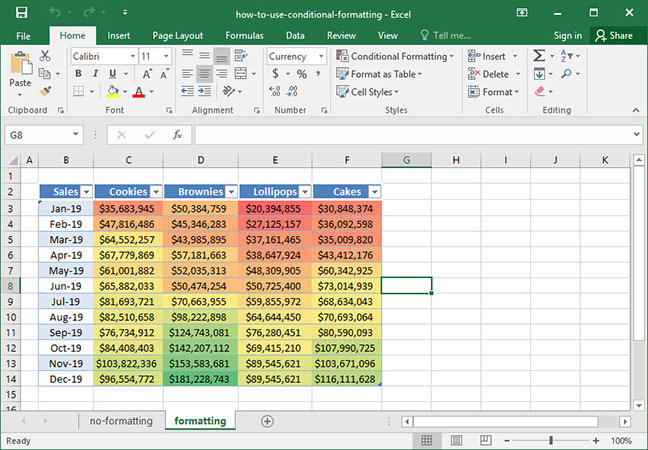
Let's take a look at a common example of conditional formatting in practice to get a first-hand view of just how useful it is. Take a look at the below spreadsheet, prepared by a SnackWorld analyst. It shows the company's total monthly sales by product category for the year of 2019:

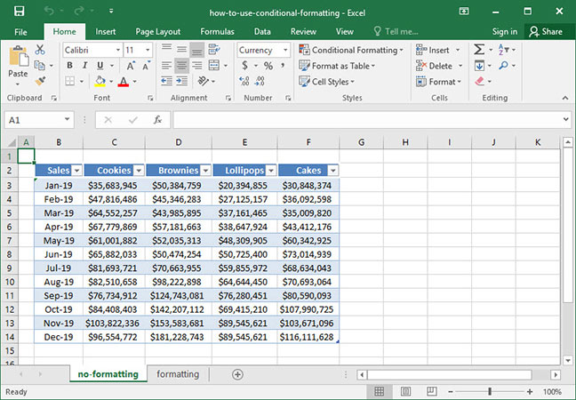
The SnackWorld CEO, upon seeing this data, had an important comment: the information is all there, but it's very hard to read the chart and identify trends without spending a significant amount of time looking at the numbers. Our analyst could create a chart or graph representing the data, but she wants to preserve it in table form so that exact sales numbers for each category and month can quickly be pulled. Is there an easy way that we could make this data easier to look at while preserving its integrity?

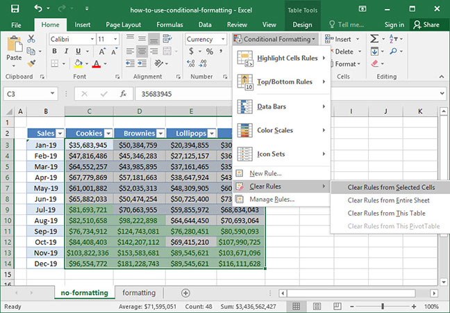
The answer is conditional formatting. Let's test it out by highlighting our data set — excluding the dates on the left-hand side of the chart, because we do not want to format those — and clicking the Conditional Formatting button on the Home tab of the Ribbon:

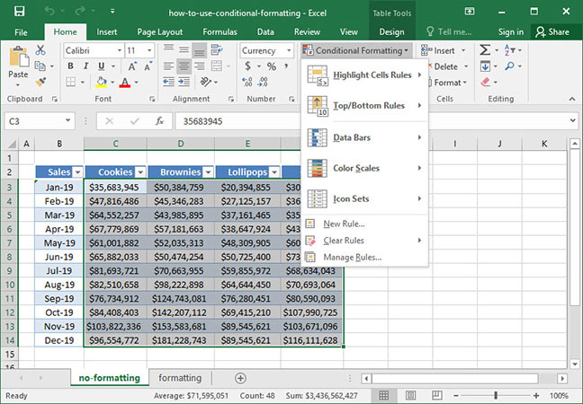
A large formatting menu opens up giving us several options:

• Highlight Cells Rules allow us to highlight particular cells based on the values that they contain. We can specify criteria telling Excel to highlight cells that contain values greater than or less than a certain threshold; between two numbers; equal to a certain value or string; containing a given substring; and more.
• Top / Bottom Rules allow us to highlight particular cells that are important relative to other values in our data set. For example, we could highlight the ten largest or smallest cells by value; the top or bottom 10% of cells by value; or cells containing values greater than or less than the data set average.
• Data Bars show values relative to the whole data set using a graph-type visual overlay.
• Color Scales change the background color of cells based on the values that those cells contain on a scale. Color scales use color gradients, with the highest-value cells appearing at one end of the gradient spectrum and the lowest-value cells appearing at the other end.

For our analyst's purposes, the Color Scales option will work the best to show our data. Let's select it and choose one of the color scales available. The first option, which we'll choose, highlights the highest-value cells in green, the middle value cells in yellow, and the lowest-value cells in red.

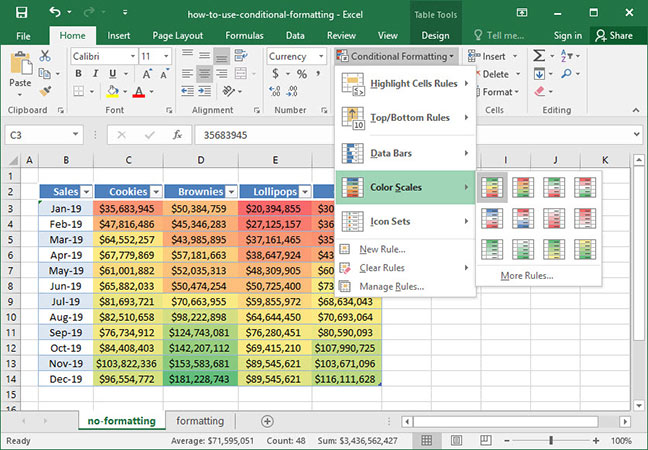
When we select this color scale, Excel tints our cells on a spectrum, with the highest values in green and the lowest values in red. Note that the program automatically uses a gradient, making it very easy to tell where our data values fall in the range.

To clear conditional formatting, select all formatted cells and look at the Clear Rules menu in the Conditional Formatting dialogue:

Those are the basics of conditional formatting, but there's much more to learn. Check out our full conditional formatting tutorial for more information!

Further reading

• How to use Conditional Formatting

There you have it: the top ten places to start when you're learning how to use Excel. We hope that this tutorial has been helpful as you start off with this amazing and powerful program. Our website features dozens of free, easy-to-follow courses on how to use Excel's formulas, functions, and other features, so be sure to check it out for more information as you learn. And if you have any questions or comments for us, we'd love to hear them — sound off in the Comments section below. Thanks for coming by!

Comments