How to alphabetize in Excel: A complete guide to sorting

One of Excel's most powerful features is the ability to quickly and easily sort data. This includes both alphabetizing lists of strings (i.e. putting them in alphabetical order), and ordering numerical values — both from largest to smallest and smallest to largest.

In this article, we'll take a look at how to do so, covering everything from standard alphabetization (sorting from A to Z) to reverse alphabetization (sorting from Z to A) to sorting numbers.

Defining the problem

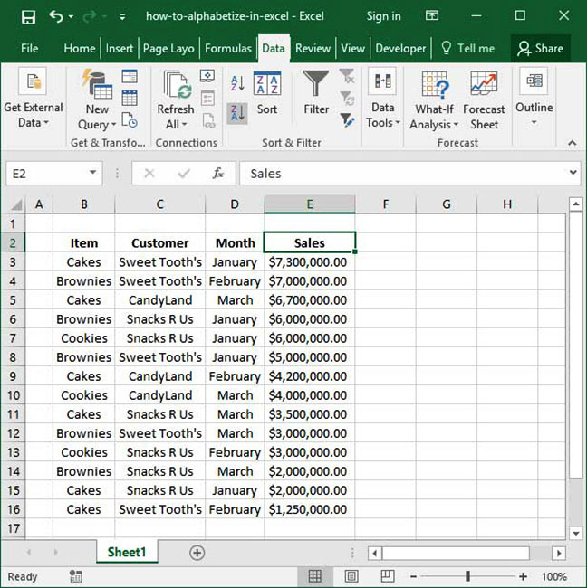
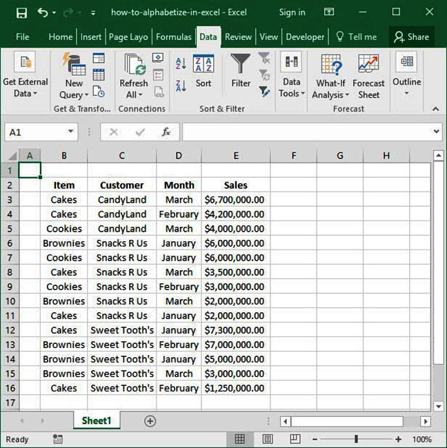
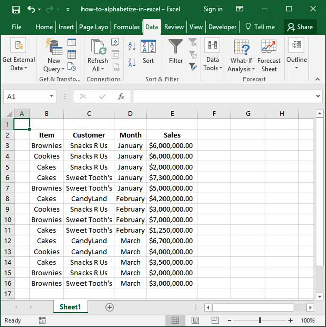
Take a look at the spreadsheet below, which shows orders from SnackWorld's customers between the months of January and March:

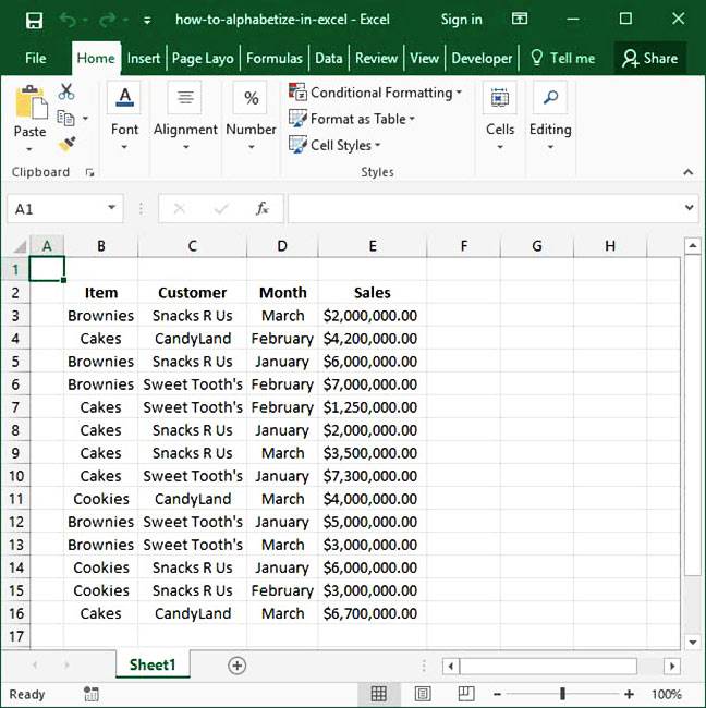
As you can see, the list is pretty messy right now. If you wanted to look up a particular customer's order history, it'd be a real pain to comb through the whole list and note each individual instance of that customer's name.

But there's a fix: if we alphabetize the list, it'll be a lot easier for us to read — and a lot more user-friendly for other folks who want to use the same sheet. Alphabetizing will have numerous advantages:

• It will make it easier for a human to look up a particular value or customer name;
• It will help us manually scan for duplicates in case we've made a data entry error;
• It will help others who use the spreadsheet understand it faster and with less effort; and
• It will allow us to easily group the orders for any particular customer together so that we can see them side-by-side.

Quick alphabetization and sorting

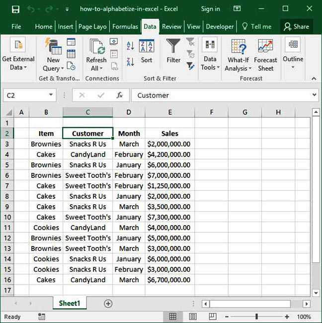
To start off, we'll use an Excel feature called Quick Sort, which allows very rapid alphabetization or ordering of columns based on a single button press.

To get started, make sure you've highlighted a cell in the column by which you'd like to sort. In this case, we want to sort by Customer, so we'll select cell C2. Next, select the Data tab on Excel's ribbon. A new set of commands will appear that are centered around editing and modifying data:

Finally, press the sort ascending button in the toolbar; it's the one with the 'A' and 'Z' (indicating alphabetization) next to a downward-pointing arrow. When you press the button, you'll see that the cells in our sheet quickly rearrange themselves alphabetically:

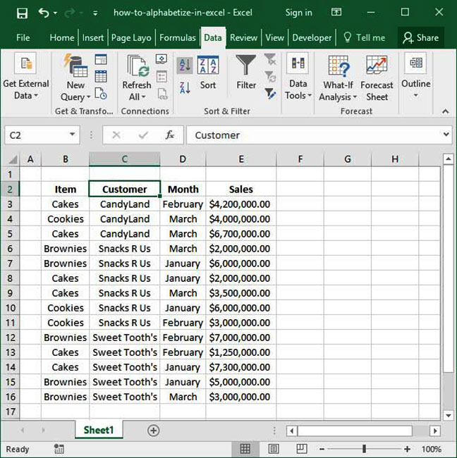
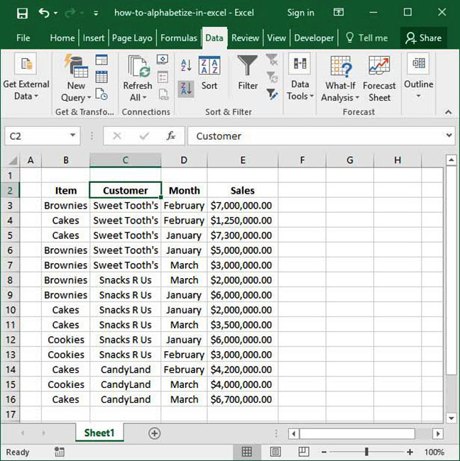
Notice that there's a very similar icon with a 'Z' first and then an 'A'; use this icon to sort descending, like so:

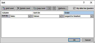
Let's say we actually want to sort by something else. For example, what if, rather than alphabetizing our list by customer, we wanted to sort it by the Sales amount to find the highest- and lowest-value orders in our data set? Doing so is easy: simply select a cell within the Sales column (we use E2 in the example below) and press the sort descending button again:

In this case, we've sorted by our sales values in descending order. The sort buttons work on numerical values as well as text!

Alphabetization by multiple columns

Now, it's time to get fancy. We know how to sort and alphabetize by a single column. But what if we want to sort by multiple columns — for example, alphabetize our order list by customer name first, but within each "customer name" block sort from the highest-value order to the lowest-value order?

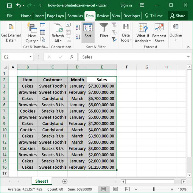
We can do this by using Excel's full sort functionality. First, we'll start by selecting the whole range of data we want to sort. You can do this by clicking and dragging with your mouse to select all the cells you want to sort, but there's a shortcut: make sure a cell within your data table is selected, then press Ctrl + A on a PC or ⌘ + A on a Mac.

When you make this selection, it's very important to check to ensure that your entire table is highlighted before proceeding. If there are blank rows, they may cause the Ctrl + A shortcut to only highlight part of tht table; this will mess up your sorting or only partially sort the data. Always double-check to ensure that your whole data range is highlighted before proceeding with alphabetization and sorting.

Next, press the large Sort icon in the Data ribbon:

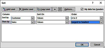
Pressing this button will bring up the Sort dialogue, a screen that will allow us to sort our data using multiple levels of specificity. The sort dialogue looks like this:

You'll notice that Excel gives us a couple of options for alphabetization in this dialogue:

• Column. This is the column that you'd like Excel to alphabetize or sort by. In this case, let's select "Customer", since the first things we want to do is alphabetize our list by customer name.
• Sort on. This is the characteristic of the cells in the given column that we would like to sort based on. We'll almost always keep Values selected in this dialogue; although once you start experimenting with more advanced sorts you can also choose to sort by Cell color, Font color, and Cell icon. For now, just leave Values selected.
• Order. This allows us to choose whether we want to sort ascending or sort descending. In this instance, let's leave the order set to A to Z to alphabetize our list in an ascending manner.

If we just pressed the OK button now, our list would sort ascending, just like we did before with the quick sort icons. But we're going to go a little further by adding another level of sorting.

First, click the Add Level button in the top-left corner of the sort dialogue. You'll see that another line, labeled Then by, appears:

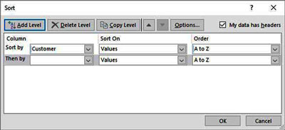
Using this second line, we can choose a second level of sorting that will occur after our data is alphabetized by customer name. Input the following into the boxes on the second line, like so:

• Column. Use Sales, because we want to order the lines in our table by sales value after we have alphabetized by customer name.
• Sort on. Leave this set to Values, as we'll do in the vast majority of cases.
• Order. You'll notice that since we have the Sales column selected, the options in this box have changed; Excel recognized Sales as a number, so it gives us a new set of options for sorting: Smallest to largest and Largest to smallest. Let's select Largest to smallest now, since we want each customer's largest order to appear at the top of its section.

Finally, press the OK button to complete the sort. Viola! Our data is now sorted in a new order: first, alphabetically by customer name; then, by sales values from largest to smallest.

Sorting or alphabetizing in a custom order

The traditional sorting methods we've been using so far present a small problem: what happens if we want to order our list chronologically by month? Our month names are entered as text strings rather than dates, so alphabetization won't work: if we sort from A to Z, February will come first, then January, then March. And if we sort the other way, March will come first, then January, then February. How can we get Excel to sort chronologically by month without alphabetizing?

The answer is simple: by using a Custom list. Try selecting your data table and opening the Sort dialogue again:

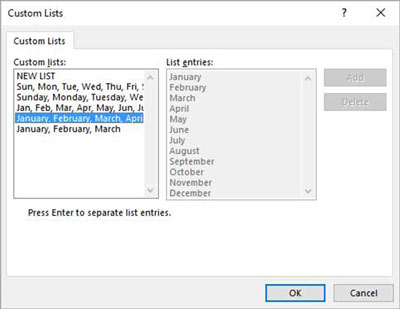
In the Column section, we'll select Month, and in the Order section, we'll select Custom List. When we do so, a new dialogue opens:

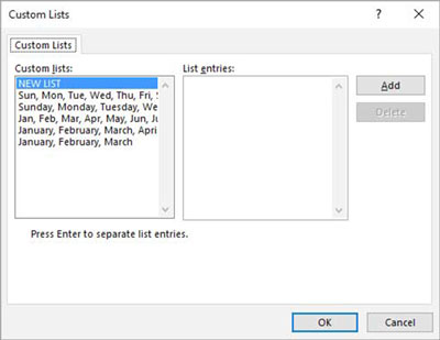
This screen will allow us to specify our own custom order of columns by typing them into the List entries section like so:

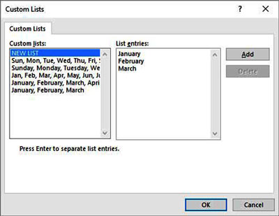
Once you've done this, hit OK to confirm our custom sort and then OK again to perform the sorting itself. You'll see that we've successfully sorted our list chronologically:

Notice that in the custom list dialogue, there are a number of presets, one of which uses the names of months in order. We can also use that preset rather than entering our own custom values. The Add button will permanently add a new custom value list you've created into the presets for future use.

Those are the basics (and some more advanced details!) on how to alphabetize and sort by values in Excel. Questions or comments on what we've done above? Be sure to let us know in the Comments section below.

Comments