Using INDEX MATCH

The INDEX MATCH function is one of Excel's most powerful features. The older brother of the much-used VLOOKUP, INDEX MATCH allows you to look up values in a table based off of other rows and columns. And, unlike VLOOKUP, it can be used on rows, columns, or both at the same time.

INDEX MATCH is so useful that many Excel pros use it to replace VLOOKUP entirely, never relying on the latter function. It appears frequently in spreadsheets, formulas, and even Excel interviews — so is a great formula to know for business analysts of any tenure.

Before we begin, it is important to realize that INDEX MATCH isn't actually a standalone function, but rather a combination of Excel's INDEX and MATCH functions. Read on to find out how to use them together to activate one of the most powerful tools Excel has to offer.

The INDEX function

We'll start with an overview of the INDEX function. Simply put, INDEX takes a cell range and returns a cell within that range based on a count provided by the user. The formula looks like this:

=INDEX(range, row_or_column)

That may sound a bit complicated, but it's actually easy once you see it in action. Take, for example, the following sheet:

=INDEX(C3:C5, 3)
Output: 9

In this example, the formula outputs the number 9, because the cell 3 spaces into the specified range contains the number 9.

Here's another example, in which we've changed the row_or_column parameter to 1:

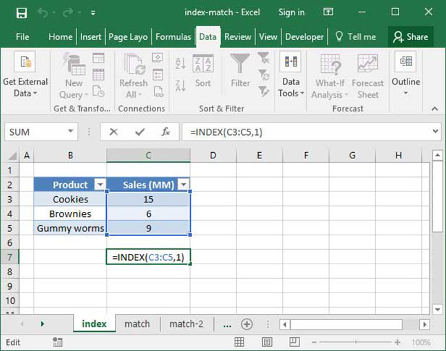
=INDEX(C3:C5, 1)
Output: 15

In this example, the formula outputs the number 15, because the cell 1 space into the specified range contains the number 15.

Let's look at one more example, in which our range is a series of horizontal cells rather than vertical ones:

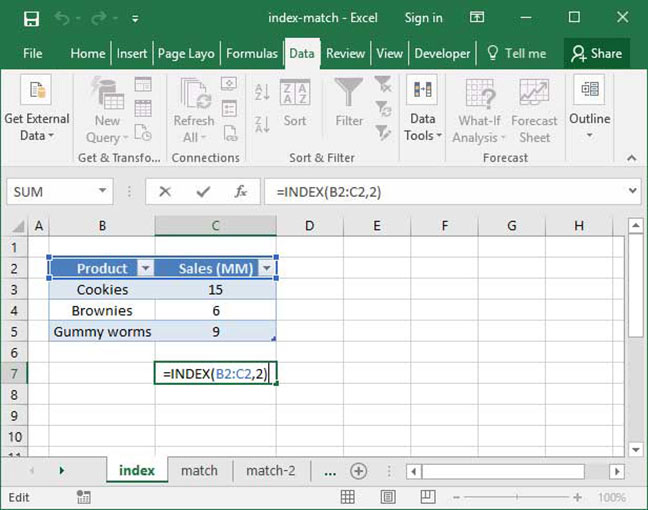
=INDEX(B2:C2, 2)
Output: "Sales (MM)"

As you can see, INDEX works exactly the same way, counting the number of cells we specify in our row_or_column parameter and outputting what it finds at the end of its search. In this case, this is the string "Sales (MM)".

This function may not seem particularly useful — and, used alone, it isn't — but when combined with MATCH, it becomes much more powerful.

The MATCH function

The MATCH function returns the position of a cell within an array by matching against a criteria string. The formula looks like this:

=MATCH(lookup_value, lookup_range, match_type)

Here's an example of MATCH in action:

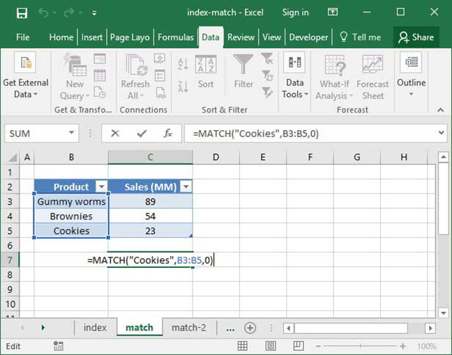
=MATCH("Cookies", B3:B5, 0)
Output: 3

In this example, the formula outputs the number 3, because the value "Cookies" is found 3 spaces into the specified lookup range.

Here's another example of MATCH used in a horizontal range:

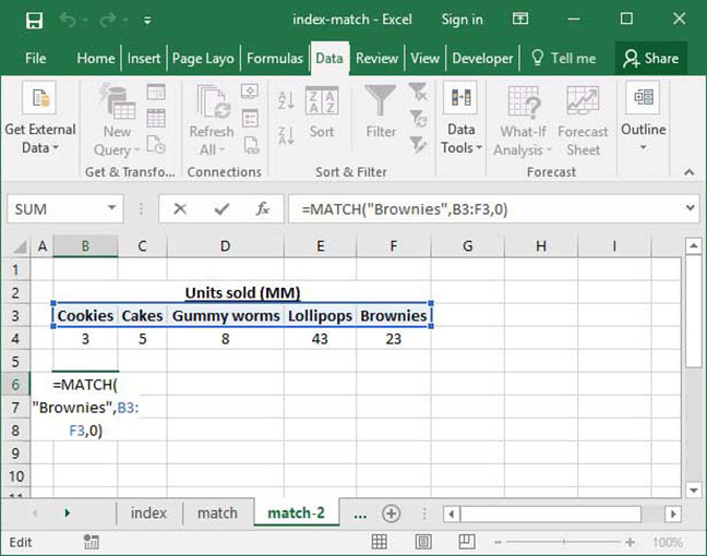
=MATCH("Brownies", B3:F3, 0)
Output: 5

In this example, the formula outputs the number 5, because the value "Brownies" is found 5 spaces into the specified horizontal lookup range.

Putting it all together

So, how do we combine INDEX and MATCH to replace VLOOKUP? We feed the MATCH function into the row_or_column argument of the INDEX function like so:

=INDEX(range, MATCH(lookup_value, lookup_range, match_type))

Let's take a closer look at what's going on here. First, we call INDEX on a range of numbers from which we would like to look up a given value. Then, we use MATCH to tell Excel how many cells it should count into INDEX's range, based on a given value matched against a separate array.

That's a lot to digest, so let's take a look at an example to make things simpler. The following spreadsheet shows SnackWorld production by month. Let's say we want to look up how many Cookies were produced in March using the following table. We could do this easily using VLOOKUP, but let's try it with INDEX MATCH instead:

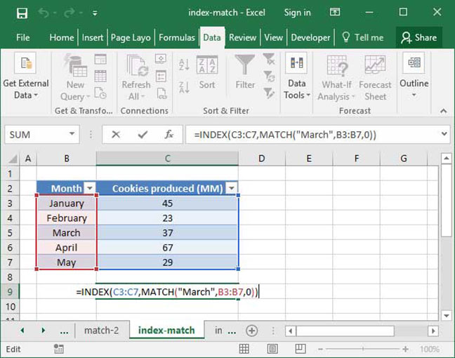
=INDEX(C3:C7, MATCH("March", B3:B7, 0)
Output: 37

In the example above, the formula outputs the number 37. Why?

First, we perform an INDEX on the Cookies produced column. How does Excel know how many cells to count down within the INDEX? It looks to MATCH, which is called on the Month column. MATCH finds the string given in the formula — "March" — three down on the list, so it pipes the number 3 back into the INDEX function, which counts down three cells and returns 37.

Let's try it again, this time with an example that will help demonstrate some of the more advanced functionality of INDEX MATCH. This time, we have a list of unit sales by category. Let's say we know one category sold 8 million units, but we're not sure which one. Let's use an INDEX MATCH to figure it out:

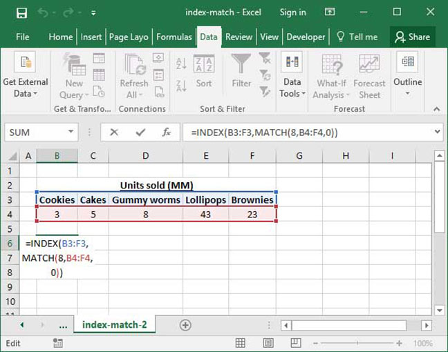
=INDEX(B3:F3, MATCH(8, B4:F4, 0)
Output: "Gummy worms"

In this case, we're using the function on a horizontal range, and we're looking up something in a table header, rather than table data itself. However, INDEX MATCH still works well.

INDEX MATCH with wildcards

You can also use INDEX MATCH with wildcards to look up based on a partial phrase or string. Take a look at our tutorial on wildcards in Excel for more information.

Why INDEX MATCH is better than VLOOKUP

After all this, you may be wondering why we even bother using INDEX MATCH. Isn't VLOOKUP just as good?

Not quite. Here are a few reasons you might want to use INDEX MATCH instead:

• You don't have to count. With INDEX MATCH, there's no more worrying about counting to figure out which column you need to pull from. You just select your lookup column and your results column, and you're done.
• You can safely insert columns. With VLOOKUP, if you insert a column in between the start of your table and the column you want to reference, your formula will break — the column_index_number within your VLOOKUP won't update. INDEX MATCH, on the other hand, safely updates no matter where you insert columns.
• You can lookup backwards. VLOOKUP only allows you to look up from columns that are in front of your starting point. Not so with INDEX MATCH — you can pull from any column you want to.
• Separate formulas. Now you don't need to remember separate formulas for VLOOKUP and HLOOKUP.
• More complex functionality. INDEX MATCH doesn't stop with the above tutorial. You can also use an INDEX MATCH MATCH to look up across both rows and columns, or use an INDEX MATCH with multiple criteria.

Now you know how to use INDEX MATCH! When you're finished reading, be sure to check out our overview of how to use Excel for more useful tools.

Comments