How To Do A VLOOKUP: The Ultimate Guide

If you've spent time with Excel, you've probably heard of VLOOKUP. It's one of the most popular and useful functions you can use on a spreadsheet, and is found in most workbooks that venture beyond simple mathematical functions like SUM and AVERAGE. It makes appearances worldwide in Excel interviews and even analytical assessments like the Uber Excel test. What is this ubiquitous function, and how can it help you save time?

In short, VLOOKUP allows you to look up a value from a separate table based on any index you choose. For example: You could dynamically look up the price of a specific item based on a price list; you could reference sales for a particular month based on a list of monthly revenue numbers; or, you could look up the name of a user based on their e-mail address.

That's a lot to take in, but things will become much clearer once we take a look at some examples below.

Defining the problem

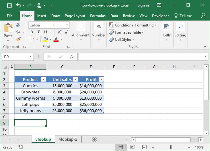
Take a look at the simple spreadsheet below, which lists SnackWorld's January sales of various types of candy.

Let's say someone asked us how many Lollipops we sold in January. To answer their question, we'd have to open up the table, scan the rows until we find the word Lollipops, and then tell them the number that sits next to it: 35,000,000.

That's easy to do when we have a small table like the one in the example above. But you can imagine it being very difficult if the table is large. It'd be a real pain to have to sift through hundreds of rows of data each time we want to look up the sales for a particular product.

That's where VLOOKUP comes in. We can use this function to dynamically look up the unit sales of a particular item from the table, based on its name alone.

Using VLOOKUP

Here's the syntax of the VLOOKUP formula:

=VLOOKUP(lookup_value, table_array, col_index_num, range_lookup)

First, VLOOKUP takes a lookup_value argument, which is a string containing the phrase that we'd like to look up — like "Lollipops", or "Cotton Candy".

Second, the function takes a table_array argument. This is the table from which we'll be looking up our values, and is specified as a cell range like B2:D7.

Third, VLOOKUP needs to know what column to pull data from. You tell it using the col_index_num argument. This argument is a number that tells VLOOKUP how many columns it should read in the table to access the data we care about. An argument of 1 will pull from the first column in the table you specify. Likewise, an argument of 3 will pull from the third column.

Finally, VLOOKUP takes a range_lookup argument. The range_lookup can be either TRUE or FALSE. If it's TRUE — or if it is omitted — VLOOKUP will assume that our input table_array is sorted in ascending order, and will find the nearest table value that is still less than the lookup_value specified. If range_lookup is set to FALSE, VLOOKUP will only return an exact match with the specified lookup term.

We almost always use FALSE as the value for our range_lookup argument, because most of the time we look for an exact match with our specified lookup term. For now, assume that you should always use FALSE as that argument, and we'll take a look at some examples later on of when you might want to mix things up!

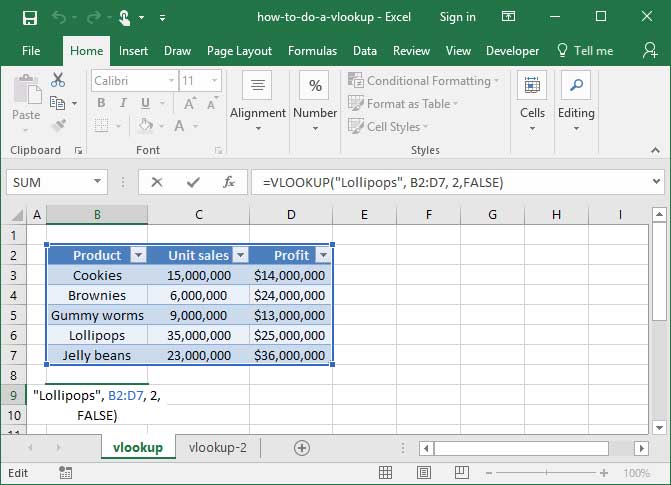
Here's a complete example of the whole formula together:

=VLOOKUP("Lollipops", B2:D7, 2, FALSE)
Output: 35,000,000

What's happening here? First, VLOOKUP looks at our table_array argument, which it sees is the table B2:D7.

Next, it looks for the lookup_value argument — which in this case is "Lollipops" — in the first column of that table. Note that our lookup value, "Lollipops", is in Column B, the first column within our table_range of B2:D7 — a critical condition for this formula to work.

Now, Excel knows that we want to pull some data from Row 6, since that's where it found the word "Lollipops" in the first column of the table we specified. To finish, it needs to know which of the other columns we want to pull data from.

So, it follows the table across col_index_num columns to find the value it's looking up. In this case, we've set our col_index_num to 2, because the Unit sales column is the second column in to the table we've specified. Therefore, the output value is 35,000,000. If we wanted VLOOKUP to return the Profit instead, we would set the col_index_num to 3, because the Profit column is the third column in to the table we've specified.

Note that our range_lookup argument is set to FALSE, so VLOOKUP will only pull an exact match to our specified lookup term.

Another example

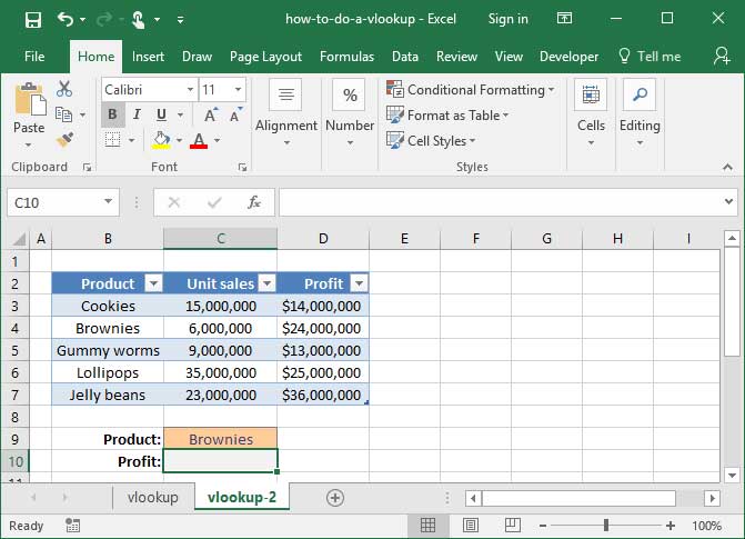
Let's check out another, slightly more complicated example of VLOOKUP. This time, we want to create a dynamic set of input fields that let us look up profit by product category automatically:

We want to write a formula in the empty grey box that will look up the Profit for whatever Product we choose. How can we do that?

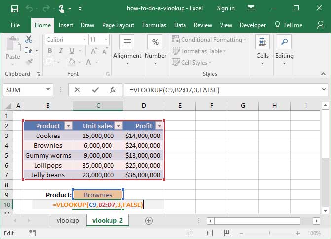
The answer: We'll use dynamic cell references within a VLOOKUP formula to reference our Product input cell. Check out the following solution:

=VLOOKUP(C9, B2:D7, 3, FALSE)
Output: $24,000,000

Let's break down what's happening here: First, VLOOKUP checks out our table_array argument, where it finds the range B2:D7. To find out which row of that table to pull, it looks to the lookup_value argument, where it finds the cell C9. Within cell C9 is the string "Brownies", so Excel uses that to identify the row we care about. Finally, VLOOKUP examines the col_index_num argument to figure out how many columns it should count in to pull data. We've told it to count in 3 columns, leading it to the Profit heading and a final output value of $24,000,000.

Now you can see how powerful VLOOKUP is — it will allow you to look up any value, in any column, off of any table, with dynamic inputs that help identify the row you care about. There are infinite applications for this capability, and we hope that this tutorial helps you find some great ones!

VLOOKUP with wildcards

You can also use VLOOKUP with wildcards to look up based on a partial phrase or string. Take a look at our tutorial on wildcards in Excel for more information.

Comments